The browser viewer

vibe-view open starts a local web server and opens the interactive viewer in your browser. This page is the reference for that surface: what is on screen, what every panel does, and the controls each section kind exposes. For a guided first look, read the walkthrough instead.

vibe-view open water.qvf
vibe-view open structure.xyz density.cube     # loose files convert in memory
vibe-view open a.qvf b.qvf                    # a Files dropdown switches between them
vibe-view compare a.qvf b.qvf                 # the same, with compare mode on

Needs the [viewer] extra (the default modes profile has it) and a browser with WebGL. The server binds to 127.0.0.1:8080 and runs until you press Ctrl+C in the terminal; it has no idle timeout.

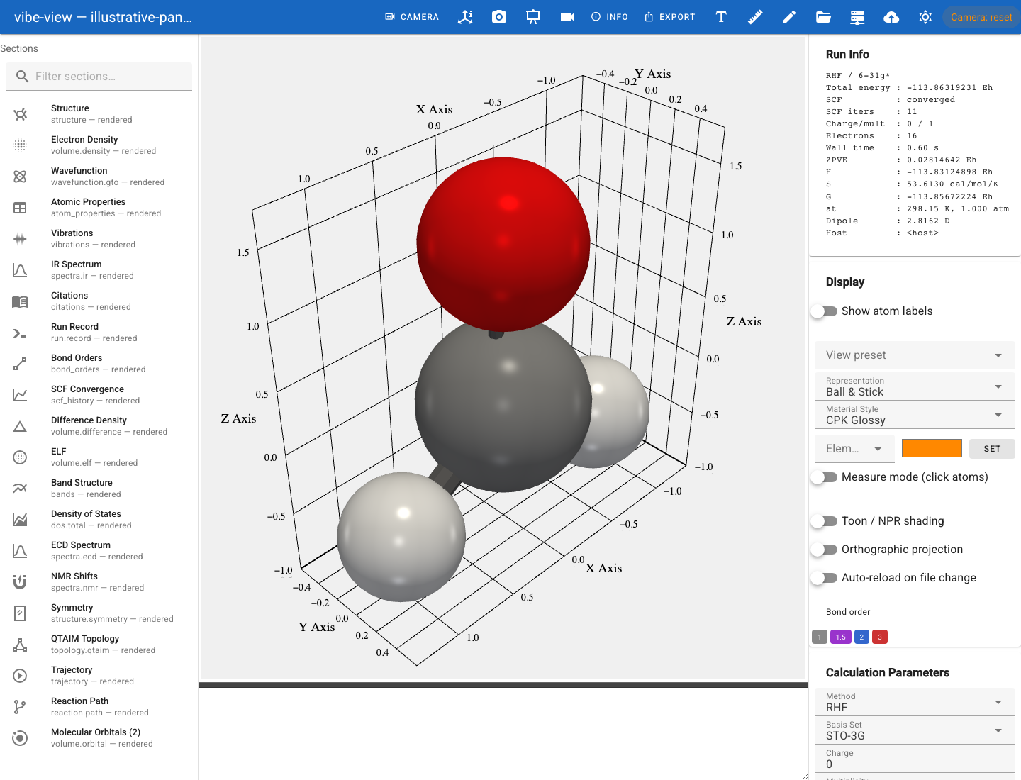
The browser viewer: the section sidebar on the left, the 3-D viewport in the centre, the per-section controls in the right drawer, and the source banner across the top.

The figures below are captures of the real viewer. Captions distinguish computed showcase data from illustrative panel fixtures.

Launch options

Flag	Effect
--port N	Bind to another port. 8080 is the default, and open refuses to start on a port something else already holds.
--host ADDR	Bind to another interface. The default is localhost only; see the warning below.
--no-browser	Start the server without opening a browser tab.
-s ID, --section ID	Activate a named section on startup.
--auto-compare	With several files, start in compare mode.
--log-file PATH	Write the server log somewhere other than ~/.cache/vibe-view/vibe-view.log, which rotates at 5 MiB with three backups.

Warning

--host 0.0.0.0 exposes the server on every reachable interface, and the server has no authentication. On a remote machine, keep the default bind and tunnel instead:

ssh -L 8080:127.0.0.1:8080 you@remote-host
# on the remote host:
vibe-view open results.qvf --no-browser

then open http://127.0.0.1:8080 in your own browser. If you only need to look, terminal mode needs no tunnel at all.

Defaults for the port, the bind address and whether a browser opens can be set once in the configuration file.

The startup banner

Before the server starts, the terminal prints one line per section saying what the viewer will do with it:

╔══════════════════════════════════════════════════════════════════════════════╗
║  QVF file: water.qvf                                                         ║
║  Source:   vibe-qc <version> - water                                         ║
╠══════════════════════════════════════════════════════════════════════════════╣
║  Section ID         Kind                         Status                      ║
╠══════════════════════════════════════════════════════════════════════════════╣
║  structure          structure                    rendered                    ║
║  density            volume.density               rendered                    ║
║  homo               volume.orbital               rendered                    ║
║  ir                 spectra.ir                   rendered                    ║
║  x_custom.notes     x_custom.notes               skipped, vendor namespace   ║
╚══════════════════════════════════════════════════════════════════════════════╝

The statuses and what they mean are listed under What vibe-view can show you. A section the viewer cannot draw still appears in the sidebar, greyed, with that reason; nothing is silently dropped, and an unknown kind never stops the rest of the file from rendering.

What is on screen

• App bar. The source banner (program, version, calculation), the Files dropdown when more than one archive is open, and the toolbar icons: open a file, edit mode, measure mode, camera views, screenshot, video export, presentation mode, the vq Job Manager, settings, and ? for the shortcut list.

• Sidebar (left). The section tree. Clicking a section makes it the active section and, for volumetric kinds, reads its payload from the archive for the first time. The Display card at the top holds the controls that apply to the whole scene.

• Viewport (centre). The 3-D scene for structures, volumes, trajectories and vibrations; an interactive Plotly chart for bands, DOS, spectra and SCF history; a table or text pane for the tabular and provenance kinds.

• Right drawer. The controls for the active section, and the cards that are only relevant in some states: Compare Files, Density Difference, Bookmarks, Calculation Parameters, Submit to vq.

• Status line (bottom). What the viewer just did, and why it refused when it did. Many controls report through it rather than through a dialog: a representation the structure cannot support, a colour mode with no data behind it, a selection that matched nothing.

A right-click on an atom opens a context menu for it, and hovering an atom shows a tooltip for it.

Keyboard shortcuts

Key	Action
Ctrl/Cmd+K	Command palette: fuzzy-search every quick action and every section by name
e	Toggle edit mode
m	Toggle measure mode
r	Reset the camera
s	Screenshot
v	Video export dialog
p	Presentation mode
Ctrl/Cmd+Z	Undo (edit mode)
Ctrl/Cmd+Shift+Z, Ctrl/Cmd+Y	Redo (edit mode)
Delete	Delete the selected atoms
Esc	Leave presentation or edit mode
← / →	Previous / next slide in presentation mode
?	Show this list in the viewer

When the command palette is open, Esc closes it and returns focus to the control that launched it, including during presentation mode.

Rotate with a left drag, pan with a middle drag, zoom with the wheel.

The Display card

These controls apply to the scene as a whole and stay put while you switch sections.

Representation. Ball-and-stick (default), space-filling, sticks only, wireframe, and cartoon for a structure that carries residues (see Biomolecules). The picker refuses a cartoon on a structure with no backbone and says so in the status line.

Material Style. Six presets: CPK Glossy (default), Matte, Glass / Translucent, Metallic, Toon / NPR and Scientific / Publication. Changing the preset re-styles every atom, bond and isosurface at once, and the background follows. A separate Toon / NPR shading switch adds outlines. View preset bundles a material, a background and label defaults into three named looks: Publication (white, clean), Presentation (dark, glossy) and Analysis (flat, labels).

Show atom labels, Orthographic projection, Dark background.

Periodic Replication (periodic files only). Nx, Ny, Nz replicate the cell along its lattice vectors. Atoms, bonds, the cell wireframe and any active isosurface expand together, and only axes flagged periodic are replicated: a slab tiles in-plane and never along its vacuum direction. Bonds that cross a cell face are drawn to the nearest periodic image rather than stretched across the box.

Auto-reload on file change. Watch the open file and hot-reload the scene when its content changes. This is how you follow a running calculation; see Jobs and live results.

Element colour override (in Settings) changes the colour of one element everywhere, including headless captures and terminal frames, so a figure made in any surface agrees with what you saw on screen.

Measuring

Press m or the ruler icon, then click atoms: two give a distance, three an angle, four a dihedral. The Measurements card lists what you have measured and can list every bond distance and angle in the structure at once. Edit mode and measure mode are mutually exclusive.

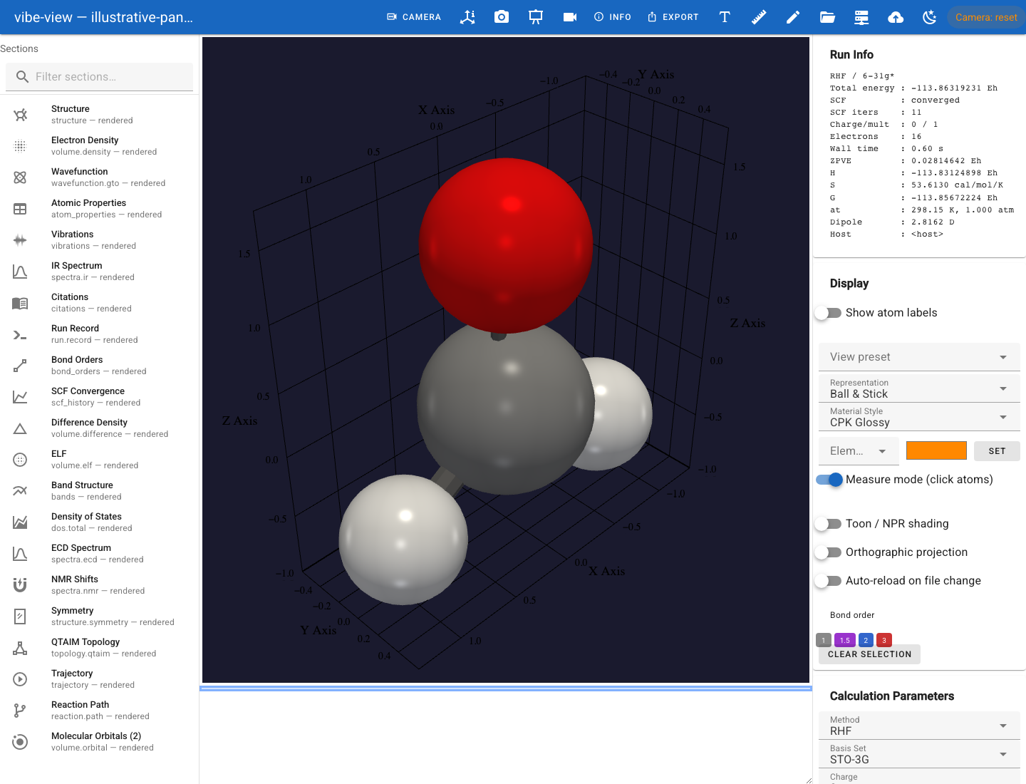
Measure mode enabled in the structure controls, ready for atom selection.

Clip plane

Enable a clip plane along X, Y or Z and drag its position to cut the scene open. It applies to atoms and isosurfaces alike, which is the quickest way to see the inside of a density surface or a cage.

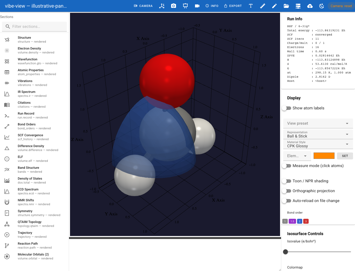
A clip plane through a density isosurface. This capture uses illustrative panel data.

Section by section

structure

Atoms as CPK spheres, bonds as cylinders. Connectivity comes from an explicit bonds section when the producer wrote one; otherwise it is inferred from covalent radii, and inferred bonds are a visual aid, not evidence that the source carried bond orders. Periodic structures show the unit-cell wireframe.

When several files are open, the Compare Files card appears:

• Overlay all structures draws every loaded structure in one viewport, one translucent colour per file, with a colour-keyed legend.

• Align (RMSD fit to first file) Kabsch-superposes each structure onto the first when the atom counts match, and reports the RMSD per file. With alignment off, structures sit at their stored coordinates.

Clicking any section leaves compare mode.

The Symmetry card detects the molecular point group (Schoenflies) from the inertia tensor and the symmetry operations it finds. A structure.symmetry section written by the producer is a different thing: that is the producer’s crystallographic analysis, shown on its own panel.

volume.* and basis.ao

Every volumetric kind (density, orbital, spin, elf, difference, potential, rdg, generic, and basis.ao) drives the same isosurface renderer, marching cubes over the stored grid. The Isosurface Controls:

Control	Effect
Volume isovalue	Slider over the data range. The default comes from the file’s viewer_defaults, or a kind-specific heuristic: 0.05 e/bohr³ for densities, 0.04 for orbitals.
Volume opacity	Alpha of the surface.
Show isosurface	Hide the surface without losing its settings.
Reduce detail (faster)	Downsample the grid before contouring. Worth it above roughly a million voxels.
Show as 2D slice	Replace the isosurface with a coloured planar cut through the field, positioned with the clip-plane sliders. Good for nodal planes and bonding regions.
Map ESP onto surface	With a volume.potential section in the file, colour the active density surface by the electrostatic potential at each vertex.
Wrap orbital to cell centre (cyclic cluster)	For a localized periodic orbital grid, roll the field so the orbital sits in the middle of the cell. Delocalized or already-centred fields are left alone.

Signed fields (orbital, spin, difference, potential) draw both lobes in contrasting colours. Unsigned fields get one surface.

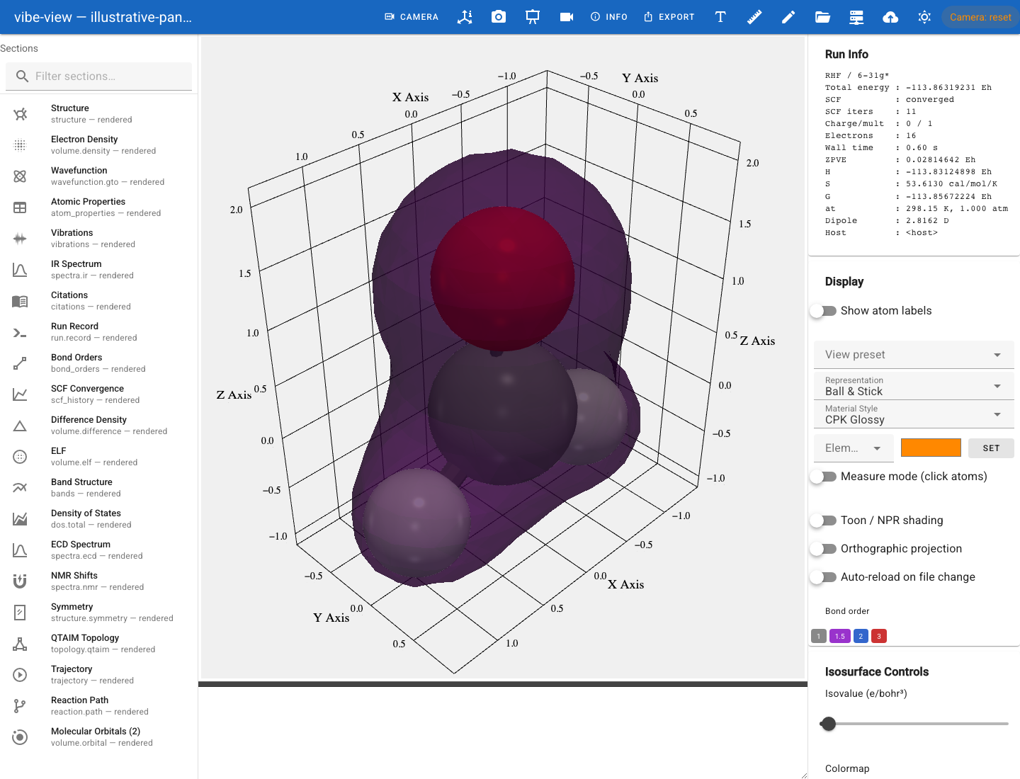
An electron-density isosurface, translucent over the structure.

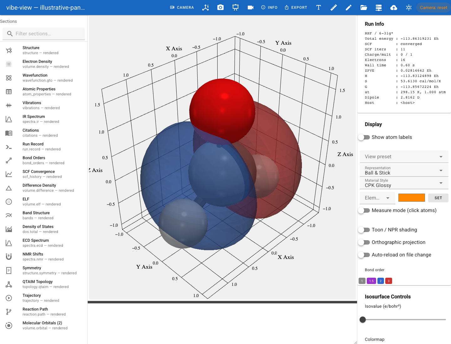
A difference density: accumulation and depletion in two colours. This capture uses illustrative panel data.

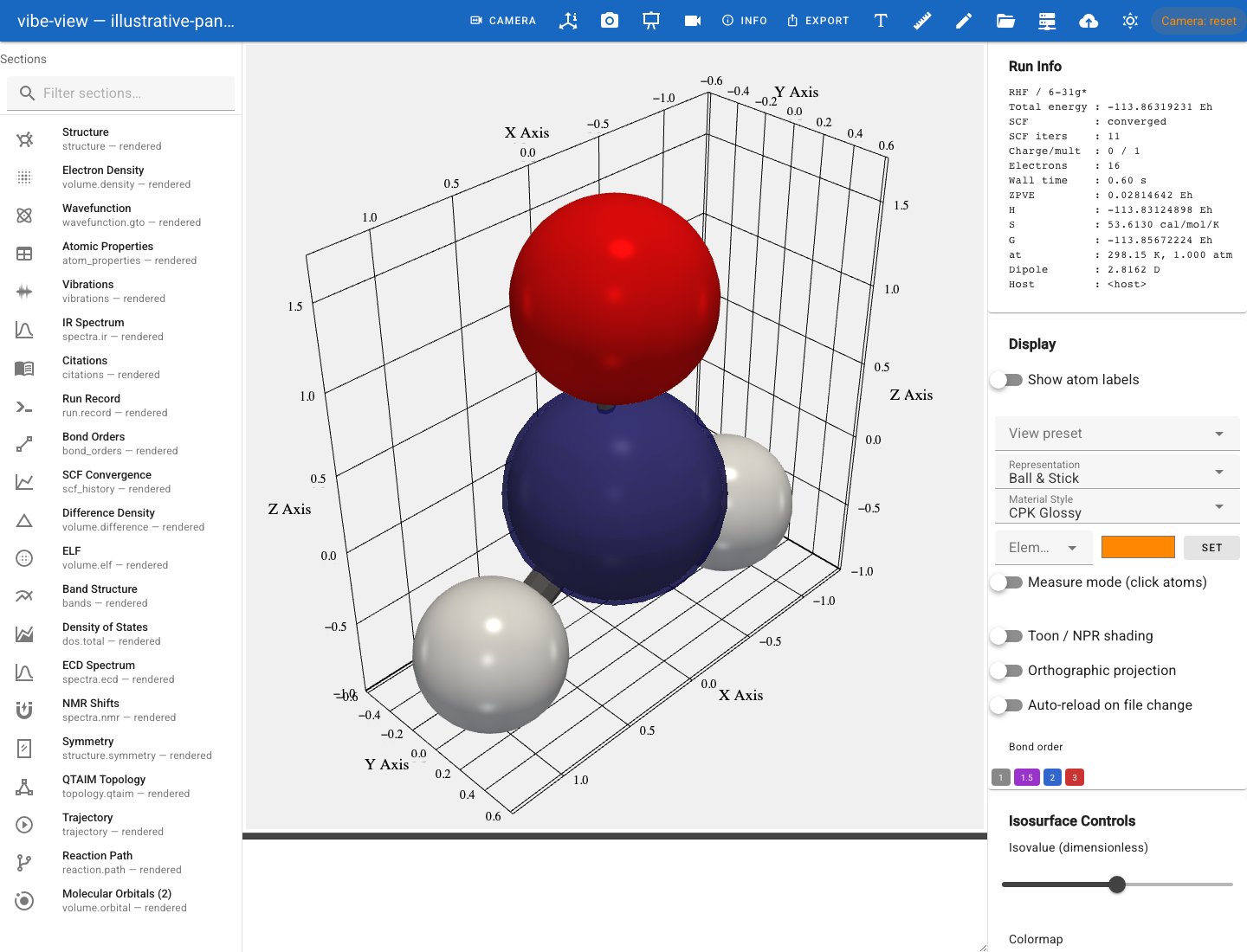
An electron localization function surface. The default isovalue of 0.8 picks out the localization basins: lone pairs, bonding regions, core shells. This capture uses illustrative panel data.

NCI. A volume.rdg section contours the reduced density gradient at s = 0.3 and colours the surface by sign(λ₂)ρ computed from a co-present volume.density section: blue for attractive, green for van der Waals, red for steric repulsion, clamped to ±0.05 a.u. With no density in the archive the surface renders uncoloured.

Cross-Fade Blend. With two volumes loaded, blend between them with a slider, which is the honest way to compare two orbitals or two densities on the same grid without flipping back and forth.

Volumetric payloads are lazy: nothing is read from the archive until you click the section, so a file with forty orbitals opens as fast as one with none.

wavefunction.gto

The Molecular Orbitals panel lists every orbital with its energy and occupation. Click a row, or use the HOMO / LUMO buttons and the previous / next arrows, and the viewer evaluates that orbital from the basis and the coefficients on a grid of its own choosing. Nothing has to be pre-computed by the producer, which is why a wavefunction.gto section is a far better way to ship orbitals than forty volume.orbital sections.

• Grid points / axis sets the evaluation resolution.

• Orbital isovalue sets the surface level; click Render MO to apply.

• Orbital component appears for complex coefficients: choose the real part (default), imaginary part, or magnitude |ψ|, then click Render MO. Signed parts use blue/red lobes; magnitude has only a positive surface. The file’s phase is preserved. An empty contour reports that the isovalue is too high for that component.

• Compute total density sums the occupied orbitals into a density surface and reports ∫ρ dV as an electron-count check.

• Canonical, alpha/beta, natural and localized sets each get their own list. Localized orbitals are labelled by the atoms they sit on, because a localized orbital has no meaningful energy ordering.

• Re-localize with sends the occupied subspace to a separately installed vibe-qc backend. Configure it as described below. IBO, Foster–Boys and Pipek–Mezey appear only when their backend readiness checks pass and the selected archive supplies compatible data.

Configure re-localization

Install vibe-qc with its native core in its own Python environment. The viewer does not need vibe-qc installed in its environment, and the backend does not need vibe-view. This integration requires the standalone worker’s API 1.0.0 or later in major version 1, JSON protocol 1, introduced for vibe-qc 0.17.5. Before that release is available, use a vibe-qc source installation containing commit 0830147b8a09f2263901960101ab571fa5e96957 or a later descendant. Follow the vibe-qc installation instructions for the native build; a Python package import alone does not establish readiness.

1. Open Settings, enter the absolute path to that environment’s Python executable, and select Save backend and check. Choose the Python executable itself, without shell arguments or a wrapper command.

2. The setting persists globally across files and viewer restarts. On startup, the viewer checks the native core and individual localization methods. Check backend repeats that probe after an installation or upgrade.

3. Select a wavefunction, keep Archived occupied orbitals selected, choose Re-localize with, then select Localize. The viewer passes exact archived shells, real occupied coefficients, occupations and structure data as JSON. It does not pass a QVF filename or reconstruct a basis by name.

For a backend Python at /path/to/backend/bin/python, these are the commands used by the viewer:

/path/to/backend/bin/python -I -m vibeqc_relocalize --probe
/path/to/backend/bin/python -I -m vibeqc_relocalize

The worker uses stdin/stdout for versioned JSON and stderr for diagnostics. The probe times out after 60 seconds; localization after 300 seconds. Cancel terminates the worker. A missing executable, incompatible protocol, unavailable native core or backend refusal produces an explanatory status in the panel.

The molecular adapter requires a restricted singlet with explicit charge, multiplicity, exact QVF GTO shells and electron occupations of 0 or 2. The occupied coefficients must cover the complete all-electron occupied subspace. No density matrix is required. A density-only archive cannot preserve the archived occupied orbitals through this interface. ECP calculations, fractional occupations, unrestricted/spinor orbitals, complex coefficients, and periodic systems (including Gamma-only archives) are not supported by this adapter. The limit is 512 AOs and elements through radon. Unsupported or incomplete archives show a reason instead of an enabled action.

New RHF + localize explicitly calculates a new wavefunction before localizing. It requires a compatible archived all-electron basis, occupations, charge and multiplicity, but does not require archived coefficients. Worker API 1.0.0 also needs the archived basis name for its atomic initial guess; exact shells still define the calculation basis. It may use edited positions of the same atoms. Changes to atom identities require a new calculation archive. Selecting this option never preserves the previous calculation’s occupied subspace, even if that calculation also used RHF. There is no automatic SCF fallback when localization fails or data is missing.

Results appear as session wavefunction overlays in the sidebar. They include localized orbital surfaces, atom populations, centroids and centre counts, plus an IAO charge table and the backend’s subspace/orthonormality errors. The viewer also checks the returned rotation and its action on the supplied coefficients. Localized orbitals have no canonical orbital energies. The panel identifies whether the source was the archive or a new RHF calculation; the current kernel does not certify localization convergence.

Clear re-localized overlays returns to the archived wavefunction. Geometry edits remove existing localization overlays. File/section changes, edits and backend changes discard any in-flight result belonging to the old state. The original QVF file is never modified. The backend’s experimental periodic finite-torus output needs additional archive metadata and a separate rendering adapter; it is deliberately not offered as molecular localization.

Orbital evaluation limits

The on-demand evaluator covers shells through l = 3. An orbital with more than 0.5 % of its weight in g or higher shells is drawn and the status line says the surface is incomplete. A wavefunction explicitly tagged with k_point: [0, 0, 0] is evaluated as a Gamma-point lattice sum in a fully periodic 3D primitive cell, including neighboring atomic-orbital tails. Skew cells keep their actual shape. Apply replication repeats that cell and its orbital surface. Very diffuse bases have a work limit; use a stored orbital grid if evaluation exceeds it.

Nonzero k-points and partially periodic Bloch evaluation are not supported and produce an explanatory error. A single stored k-point block also does not establish the weights needed for a total periodic density or its ELF/NCI/Laplacian; select the producer’s stored fields instead. Older periodic archives without explicit k-point metadata retain central-cell/cluster sampling and do not acquire a Bloch interpretation from their filename.

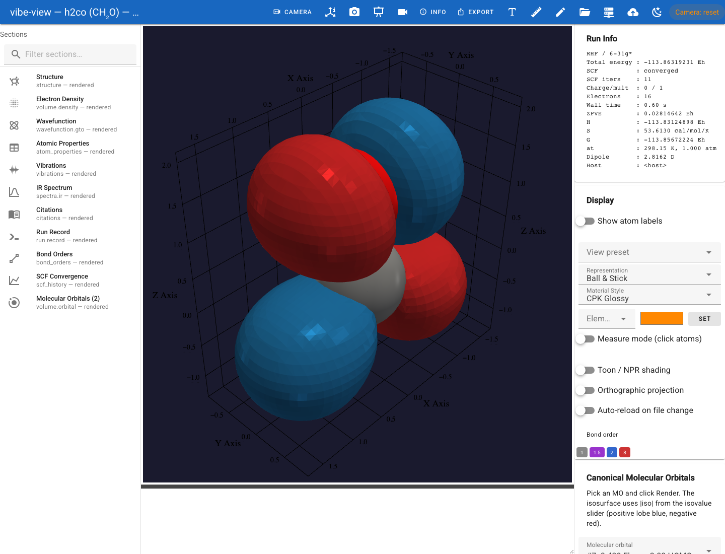
An orbital evaluated on demand from wavefunction.gto, both lobes drawn.

The Basis Functions panel does the same for a basis.ao section: pick an atomic orbital and see it.

bands, dos.total, dos.projected, dos.coop, dos.cohp

Interactive Plotly charts. A bands section plots every band along the k-path with the Fermi level as a horizontal reference; hover any band for its energy. When a dos.total section is also present the two are drawn as one figure on a shared, Fermi-referenced energy axis. Bands are shifted by their own kpath.fermi; QVF DOS grids already use E_F = 0 and are never shifted again by an absolute Fermi tag. If bands lack a Fermi reference, the panels use separate energy axes and labels. Projected DOS, COOP and COHP add per-channel traces you can toggle in the legend.

Energy window. An all-electron periodic archive carries core states hundreds or thousands of eV below E_F, and an axis autoscaled to all of them squeezes the valence and conduction bands into a few pixels. The panel therefore opens on a valence window: the states grouped around E_F, with the core shells left off the axis. E − E_F min and E − E_F max move it — commit with Enter or by leaving the field — and Reset window returns to the default. Double-clicking the chart is Plotly’s own autoscale, which shows the full range including the core states.

A file whose spectrum has no core states is not windowed at all, so pseudopotential archives keep the axis they have always had. A producer can ship its own first view with an energy_window hint in viewer_defaults, as [min, max] in eV relative to E_F:

"viewer_defaults": {
  "bands": {"energy_window": [-15.0, 10.0]}
}

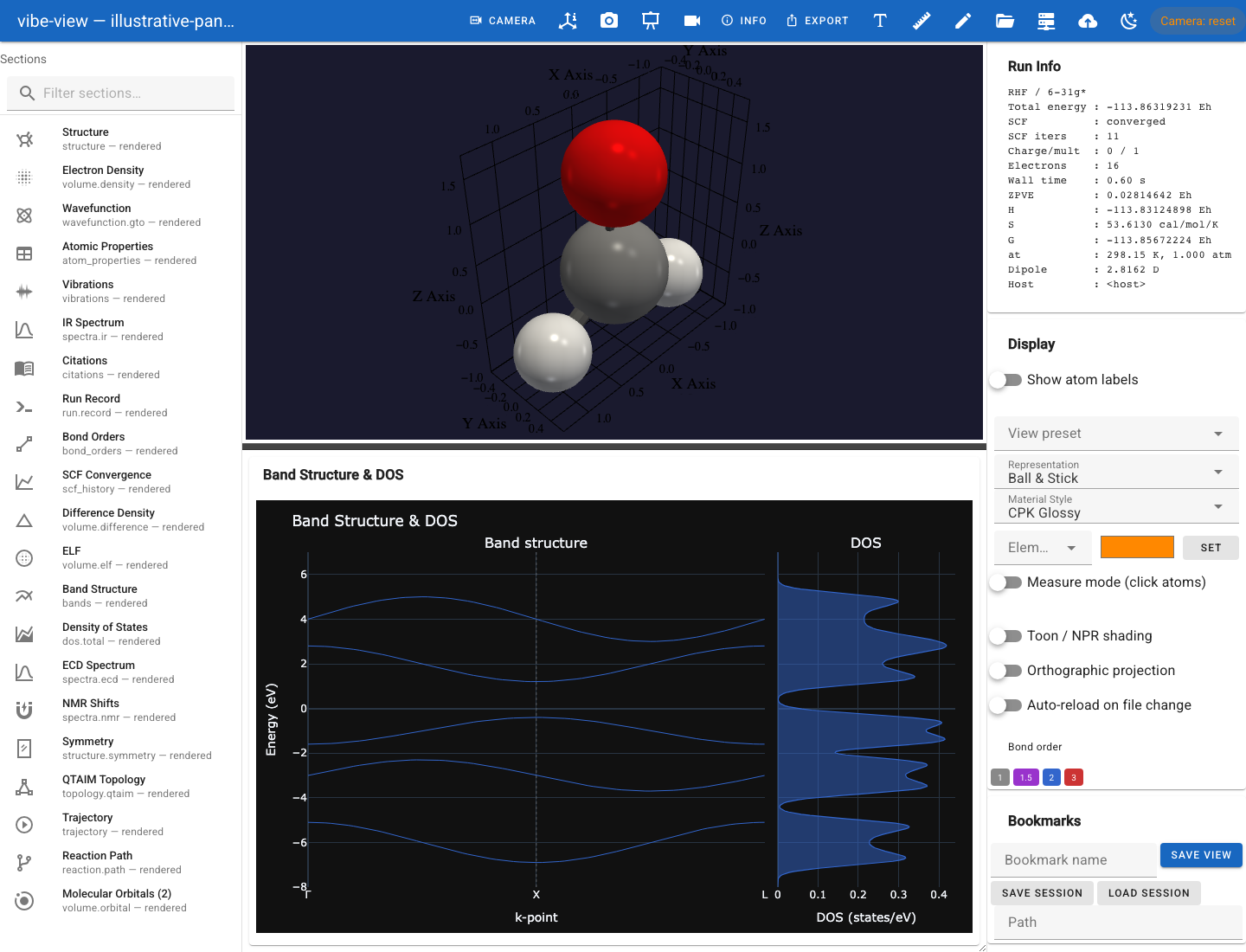
Band structure and density of states on one Fermi-referenced axis. This capture uses illustrative panel data.

fermi_surface

The Fermi surface in reciprocal space, one sheet per band crossing E_F, inside the reciprocal-cell wireframe. Because this is k-space, the real-space structure is hidden while it is shown; click any other section to bring it back. Bands shown in the Fermi Surface Bands card isolates individual sheets.

phonon_bands, phonon_dos, equation_of_state

Phonon dispersion and phonon DOS share the chart panel with the electronic bands, in cm⁻¹, and draw imaginary modes below zero rather than hiding them. An equation-of-state section plots the sampled (V, E) points, overlays the producer’s fitted Birch–Murnaghan or Murnaghan curve, marks V₀ and annotates B₀ and B₀′.

spectra.*

spectra.ir, raman, uvvis, ecd, vcd and generic render as stem charts of intensity against frequency with hover tooltips, in each kind’s native unit. Spectrum broadening draws a Lorentzian envelope under the sticks, and it is named in the legend so the convenience is never mistaken for the data; X unit and Normalize adjust the axis. Signed spectra keep their negative bands.

spectra.nmr and spectra.epr are tables: shifts and couplings, g-tensors and hyperfine values.

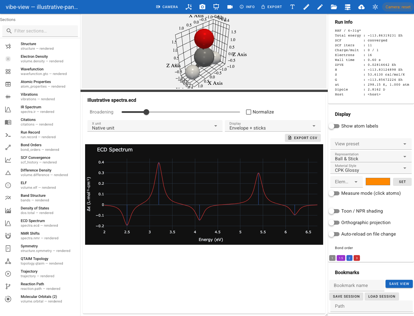
An ECD spectrum. Cotton bands of both signs are kept. This capture uses illustrative panel data.

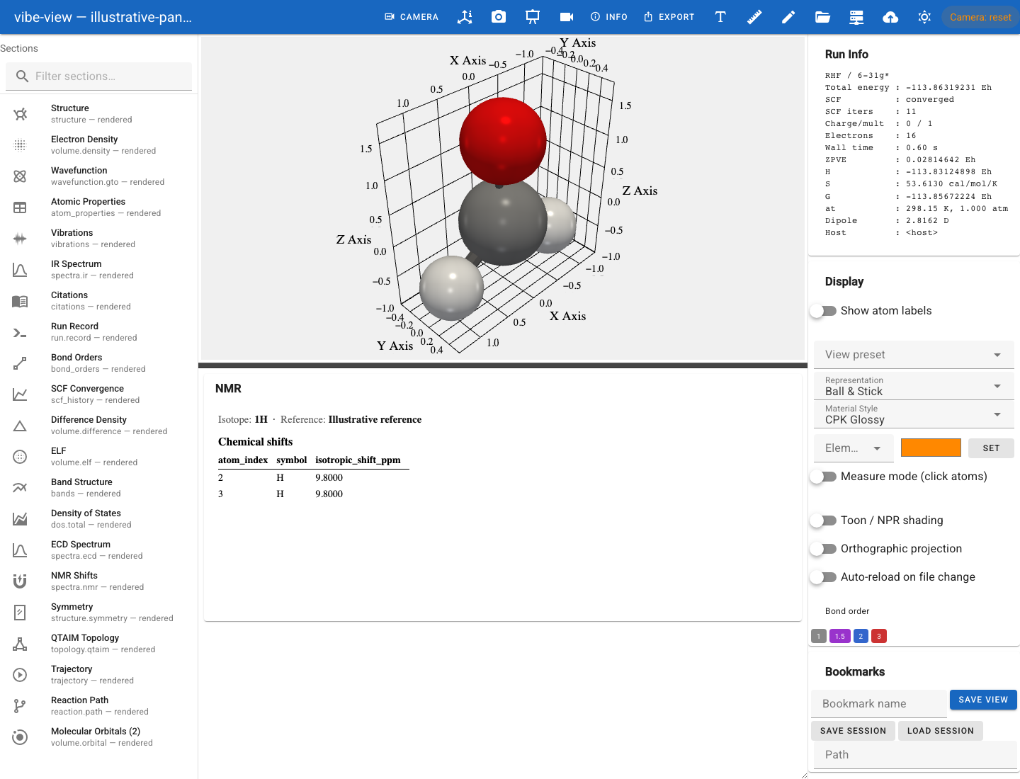
The NMR panel. This capture uses illustrative panel data.

trajectory and reaction.path

Frame-by-frame playback with a play / pause / step strip and a frame slider. Bonds are re-inferred per frame, so they follow the geometry. The Energy Profile card plots energy against frame and tracks the current frame; for a reaction path the Reaction Waypoint card names the reactant, transition state, intermediates and product as you pass them.

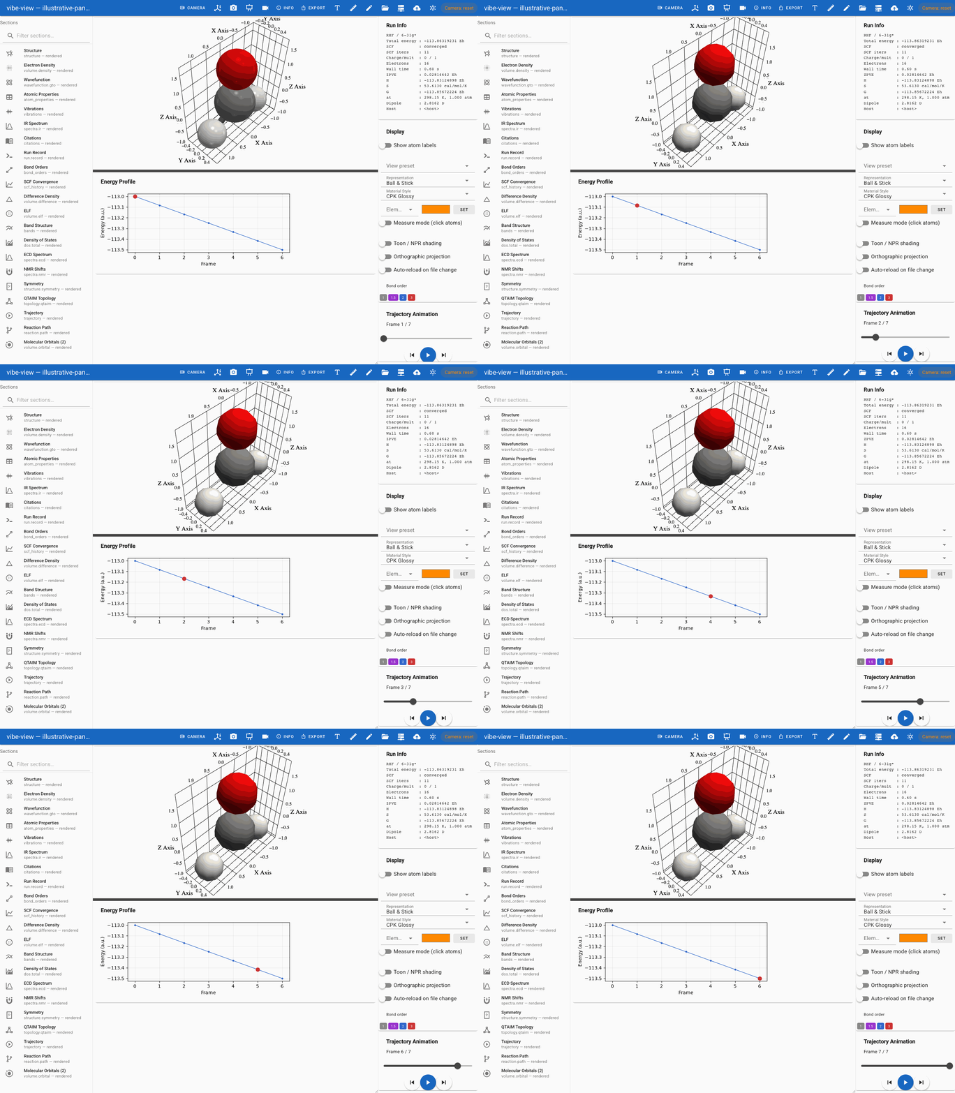
Trajectory playback with the energy profile tracking the frame. This capture uses illustrative panel data.

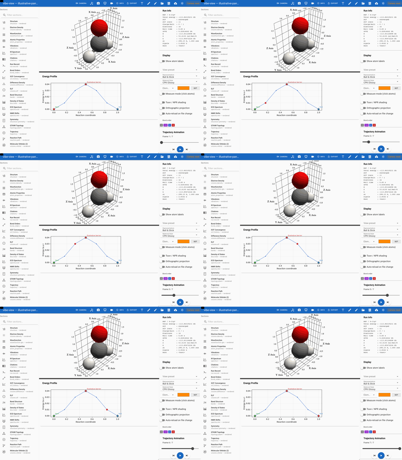
A reaction path: the waypoint label changes as the band is played. This capture uses illustrative panel data.

Periodic reaction paths carry the lattice per frame; the viewer draws the cell and wraps atoms across periodic boundaries, and a variable-cell path animates the box with the geometry.

vibrations

Pick a normal mode by frequency from the Vibrational Modes list and the structure oscillates along its displacement vector; Vibration displacement amplitude scales the motion. Mode labels carry the IR intensity when a companion spectra.ir section is present.

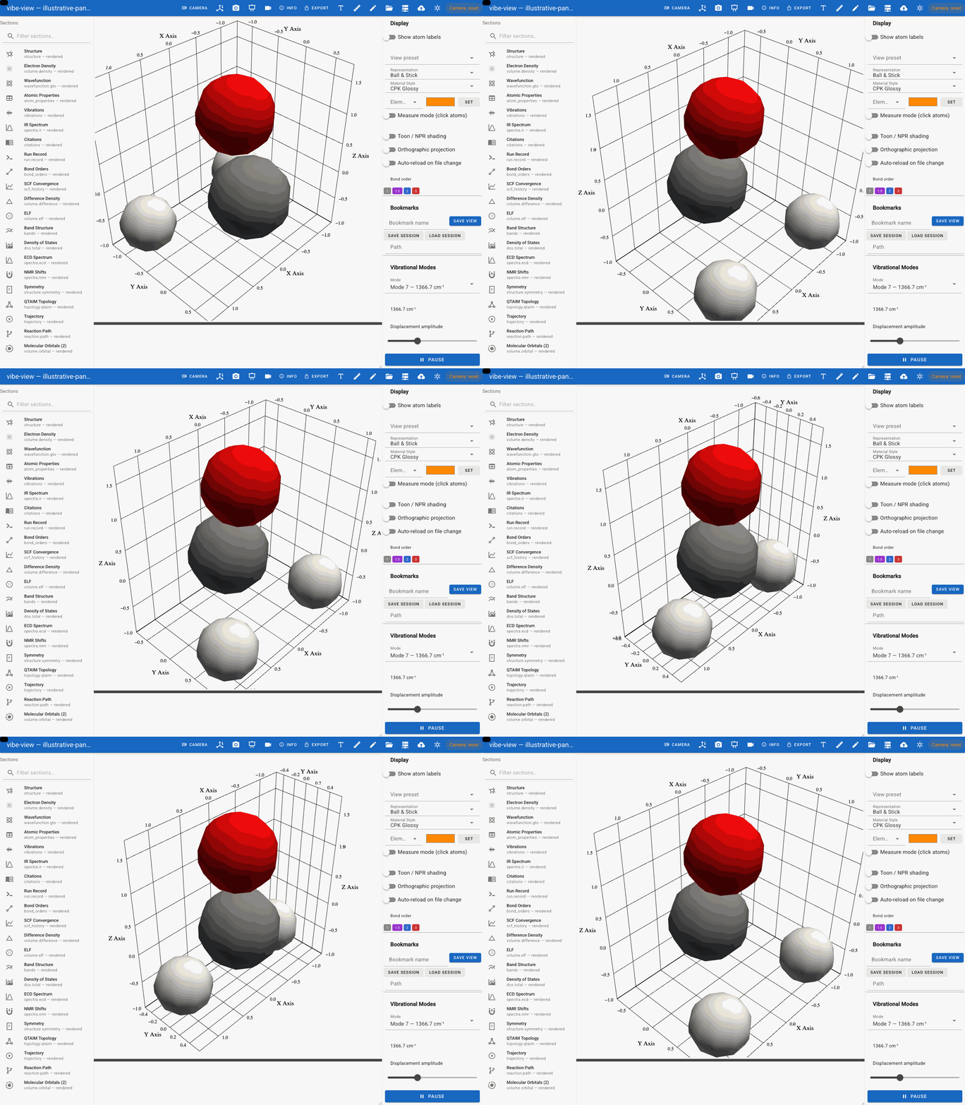
A normal mode, animated about the equilibrium geometry.

scan.surface

A relaxed or rigid two-dimensional scan, drawn as a contour surface with the two scan coordinates on the axes.

atom_properties, bond_orders, topology.qtaim

Population Analysis tabulates whatever the producer wrote: Mulliken, Löwdin, Hirshfeld charges, spin populations. Color atoms by charge tints each atom in the viewport, red positive and blue negative, and the tint follows replicas in a replicated cell.

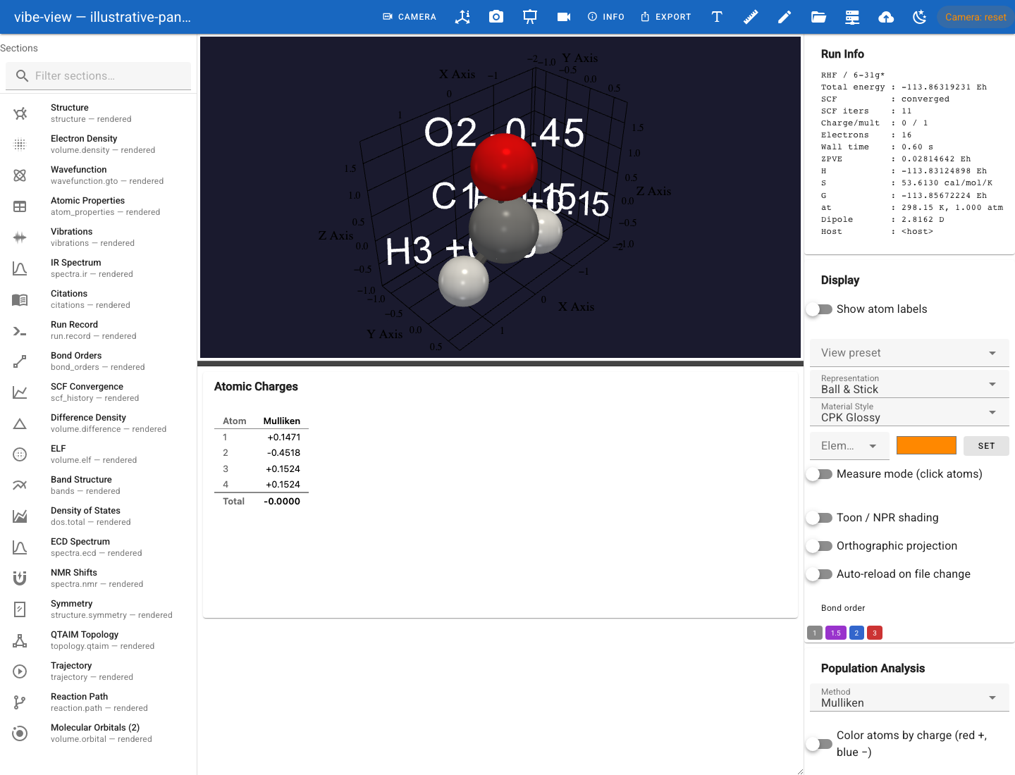
Charges as a table and as an atom overlay.

bond_orders is a triangular matrix table with CSV export, and its values colour the bonds in the structure. topology.qtaim overlays critical points as coloured spheres and draws bond paths through them; click a point for its density, Laplacian and ellipticity.

scf_history

Energy against iteration on top, DIIS error on a logarithmic axis below. Log scale (|E − E_final|) and Hide initial guess reshape the top pane when the first point dwarfs the rest.

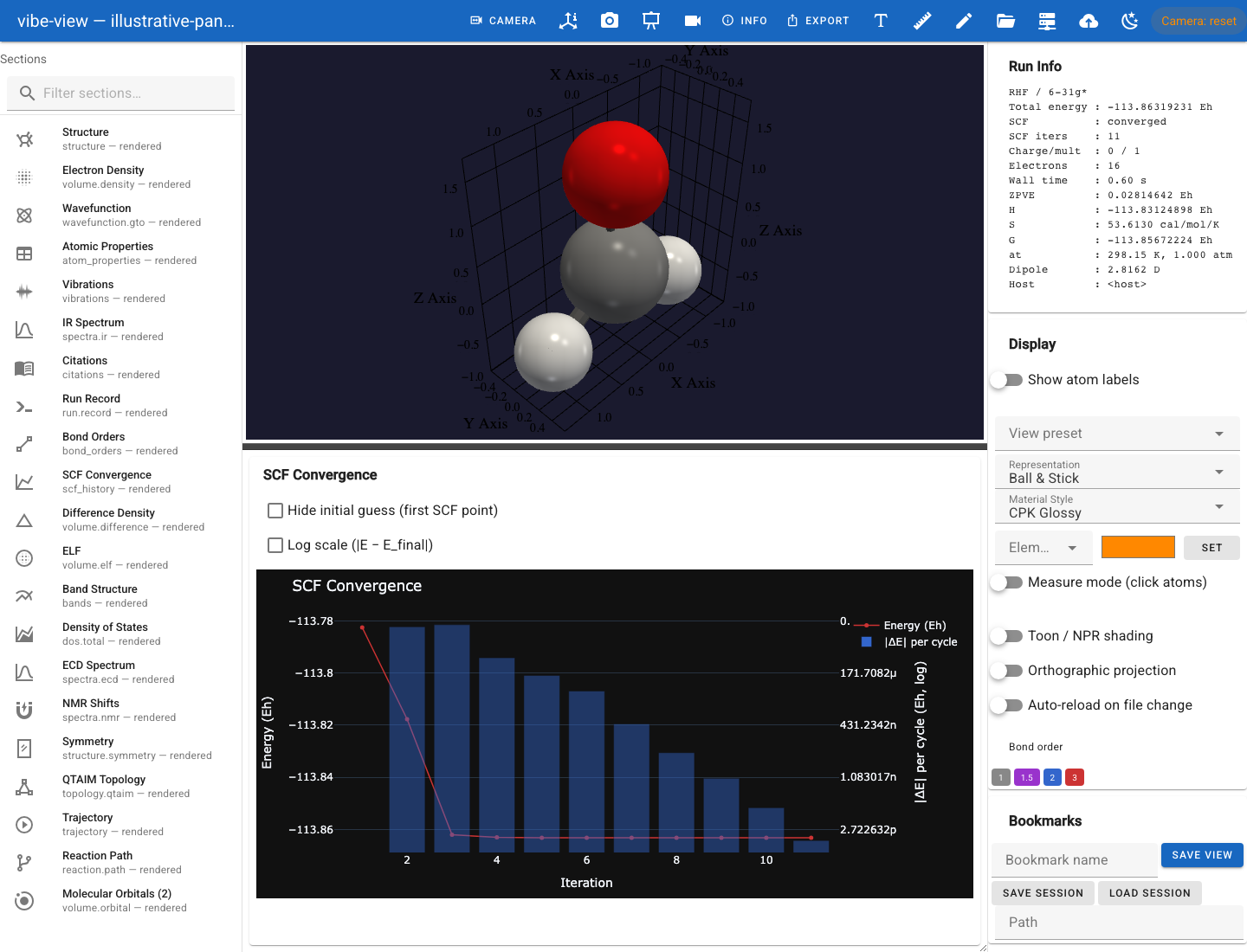
SCF convergence, iteration by iteration.

structure.symmetry

The producer’s crystallographic analysis: space group, Hall number, international symbol, Wyckoff positions, equivalent atoms.

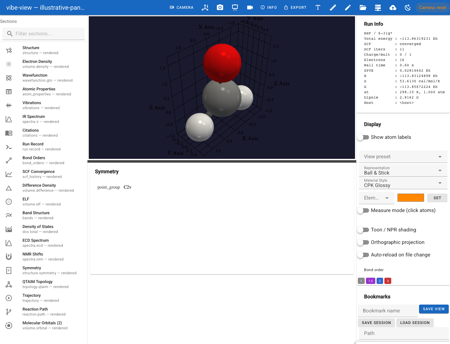
The symmetry panel. This capture uses illustrative panel data.

citations, run.record, job.spec

The embedded BibTeX bundle as a copy-paste block; the Run Info panel with the executed input, the log tail and the system manifest; and the job specification a container was built from. A container that has not yet run opens with an amber pending chip and a Job Spec panel saying so.

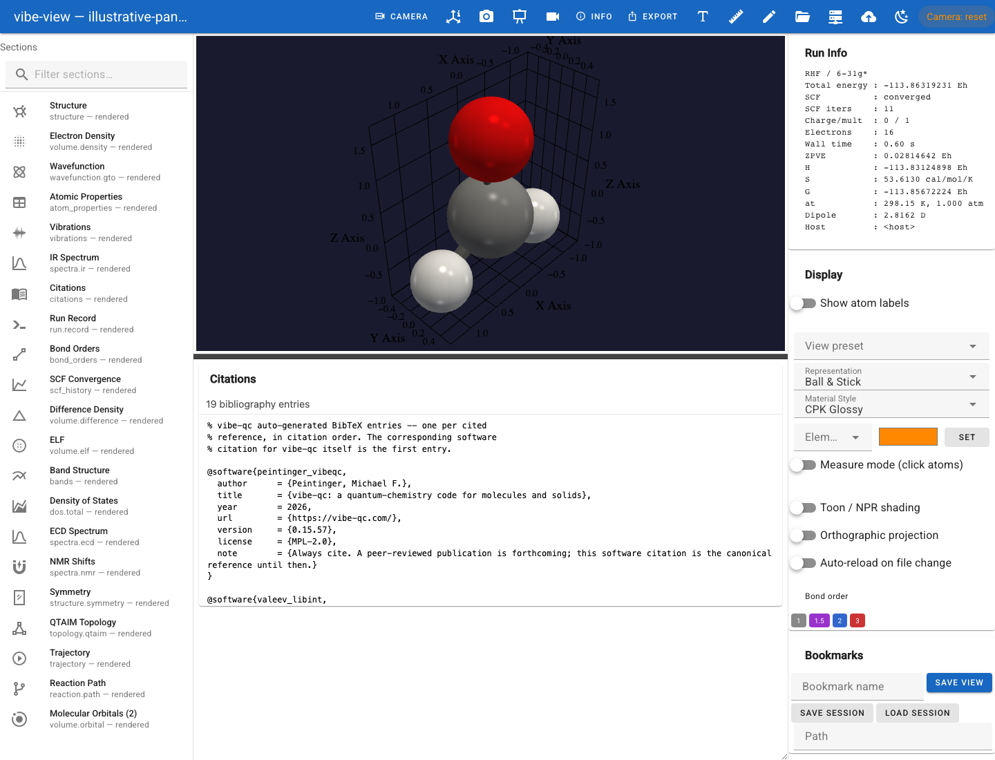
The citations panel.

Bookmarks, sessions and presentation mode

The Bookmarks card saves the current camera, active section, isovalue, colormap and opacity under a name (Save View). Selecting a saved bookmark restores all five instantly. Save Session writes every bookmark plus the current state to a .vibe-session JSON file next to the archive, and Load Session restores it; the file is plain JSON and can be version-controlled or generated by a script.

Presentation mode (p or the toolbar icon) turns the bookmarks into a full-screen slideshow: ← / → step through them, Esc leaves. Each slide restores its camera and section.

Screenshots, video and high-quality renders

Export Screenshot (s) writes a PNG at a chosen resolution and scale, optionally with a transparent background, and can save it next to the archive; Recent Exports lists what you have written. Export Video (v) renders a turntable, a trajectory, a vibration or an orbital sweep to MP4 or GIF with a chosen frame rate and quality. Both are server-side renders, so ambient occlusion and the material presets apply to them exactly as they do to vibe-view capture.

High-Quality Raytrace Render is a path-traced render with physically based materials, environment lighting and depth of field, meant for a cover figure. It appears only when the installed VTK build ships OSPRay; the card is absent otherwise rather than failing on use.

For rendering outside the browser entirely, including POV-Ray and Blender scenes, see Figures without a display.

viewer_defaults: hints from the producer

A producer can suggest how a file should open by writing viewer_defaults into the manifest: which section to activate, per-section isovalues, colormaps and opacities, camera bookmarks, and the bands/DOS energy window. vibe-view applies them before rendering anything. They are hints: every one can be overridden from the UI, and unknown fields are ignored rather than rejected. The keys are described in the QVF specification in the qvf repository.

Opening files from inside the viewer

The open dialog takes a path to a .qvf file or a directory, searches subdirectories on request, and can open a file as a separate entry in the Files dropdown rather than replacing the current one. It accepts the same loose formats as the command line; see Input formats.

When something looks wrong

The browser-specific failure modes, from a stale server behind a tab that no longer responds to the mouse to Firefox on macOS 15 refusing to connect to localhost, are collected in Troubleshooting.