Terminal mode

vibe-view show and vibe-view tui render an archive as text: the 3-D scene, the charts and the tables, drawn with Unicode braille characters and 24-bit colour in whatever terminal you are already sitting in.

The point is where it runs. The browser viewer and the headless PNG capture both drive VTK through an OpenGL context. A compute node reached over SSH usually has no display server, no GL and no X forwarding, and that node is exactly where a .qvf lands. The terminal rasterizer is pure NumPy: it paints spheres, bonds, isosurface triangles and plot lines into a depth-buffered pixel array and packs that array into braille glyphs. Isosurface extraction uses VTK’s marching-cubes filter, which is pure computation and opens no render window.

ssh compute-node
vibe-view show ~/scratch/job.qvf          # one frame, then exit
vibe-view tui  ~/scratch/job.qvf          # interactive

Two commands

	vibe-view show	vibe-view tui
Output	one frame to stdout, then exits	a full-screen interactive app
Needs	the core install: no display, no GL	the [tui] extra, which adds Textual
Good for	pipes, CI logs, scripts, a quick look	browsing an archive section by section

Both need a terminal that speaks 24-bit colour and a font with braille coverage, which most modern monospace fonts have. If the glyphs come out as boxes, add --mode half (or press d in the TUI) and the pictures switch to block characters.

vibe-view show

vibe-view show job.qvf                            # the structure
vibe-view show job.qvf --section vol_mo_3         # a specific section
vibe-view show job.qvf -s vol_mo_3 --isovalue 0.03
vibe-view show job.qvf --info                     # provenance and the section inventory
vibe-view show job.qvf --all --plain > frames.txt # every graphable section, no colour

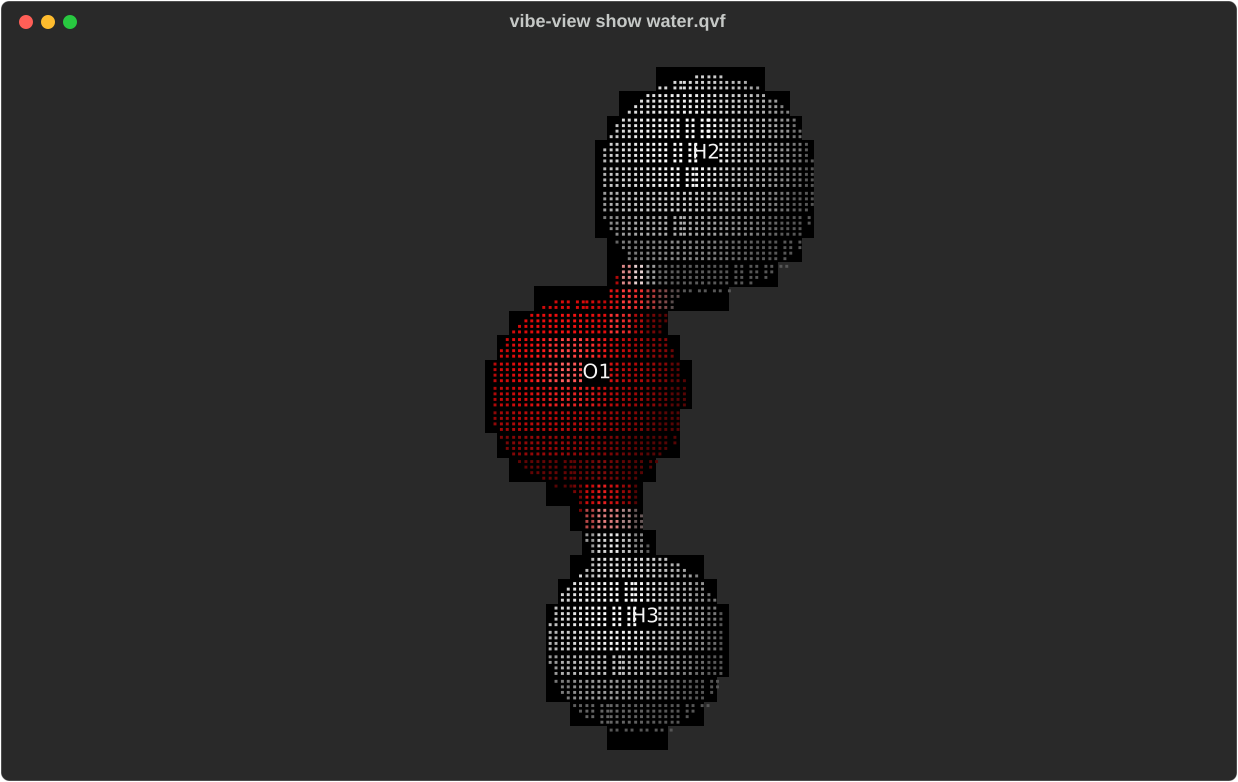
vibe-view show water.qvf --labels. Analytically shaded spheres and split-colour bond cylinders, packed into braille cells two dots across by four down, so an 80×24 terminal is a 160×96 pixel canvas.

Option	Effect
-s ID, --section ID	Section to render; the structure by default.
--all	Render every graphable section in turn.
--info	Print the archive summary instead of a picture: provenance, run lifecycle, and every section with its status from the kind registry.
--size COLSxROWS	Fix the character grid instead of asking the terminal.
--mode braille|half	See Rendering modes.
--plain	No colour, plain characters, for pipes and logs. NO_COLOR is honoured too.
--representation	ball_and_stick (default), licorice, spacefill, wireframe, points, backbone.
--color-by	element (default), chain, secondary, bfactor.
--rotate X,Y,Z	Euler angles in degrees; the default is -14,-31,0.
--isovalue F	For volume sections; default 0.05.
--replicate nx,ny,nz	Supercell view. Only periodic axes replicate.
--labels	Overlay atom indices.
--frame N	A frame of a trajectory, reaction path or normal mode.
--chart	For a reaction path or trajectory, draw the energy profile instead of the geometry.

Colour escapes survive a pipe, so vibe-view show job.qvf | less -R keeps the shading. Because it exits, show composes like any other command:

vibe-view show job.qvf --plain > frame.txt
watch -c -n2 'vibe-view show running.qvf'          # a crude live monitor

--info is the fastest way to find out what a calculation actually produced:

Archive
path                   water.qvf
qvf version            1
producer               vibe-qc

Provenance
basis                  6-31g*
functional             PBE
method                 rks
scf_converged          True

Sections
id            kind              status    note
structure     structure         rendered
density       volume.density    rendered
homo          volume.orbital    rendered
wavefunction  wavefunction.gto  rendered
ir            spectra.ir        rendered
scf_history   scf_history       rendered

The status column comes straight from the viewer’s kind registry, so a section the viewer cannot draw still appears with the honest reason.

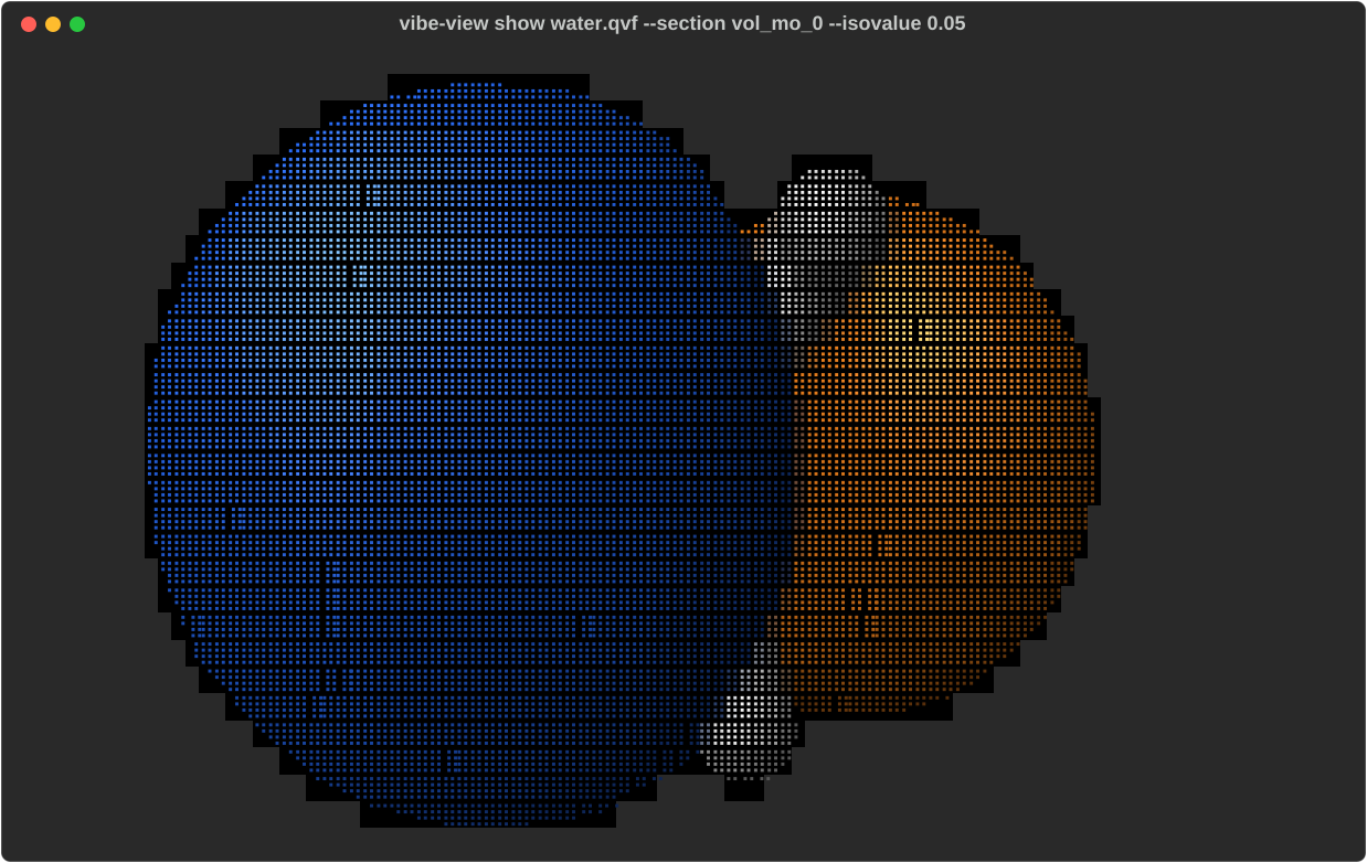
An orbital at isovalue 0.05 in licorice representation. Signed fields get both lobes, orange positive and blue negative, depth-tested against the atoms.

vibe-view tui

The interactive viewer opens on the structure with the section browser on the left, the viewport in the middle and a status line naming what you are looking at. Press ? for the key map.

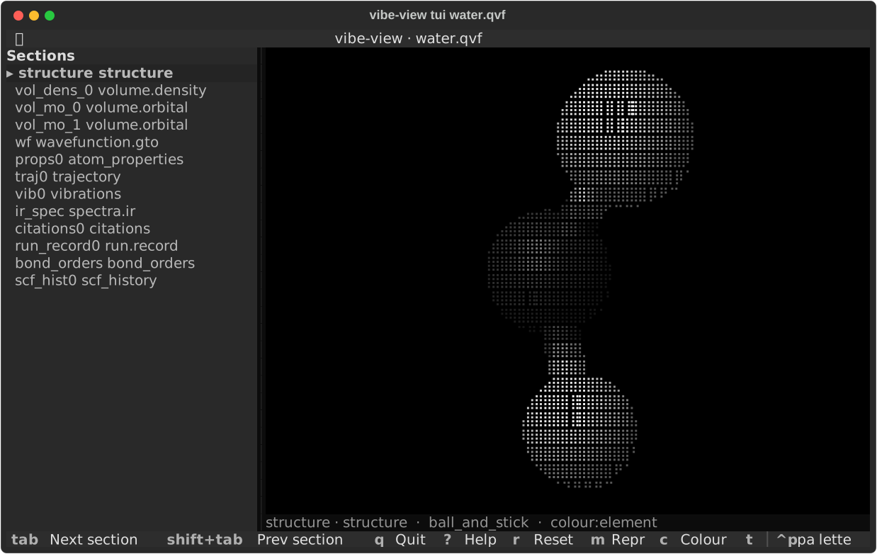
vibe-view tui water.qvf. The section browser lists every section with its status, so one the viewer cannot draw is still visible, with its reason.

Keys

Key	Action
Tab / Shift+Tab	next / previous section
arrows or h j k l	rotate
H J K L	pan
+ / -	zoom in / out
r	reset the camera and re-fit
m	cycle representation
c	cycle colour scheme
b / u / #	toggle bonds / unit cell / atom indices
d	switch between braille and half-block rendering
x y z (X Y Z)	replicate (un-replicate) along a, b, c
o	isosurface on / off
i / I	isovalue down / up
n / p	next / previous stored volume, or next / previous orbital while a wavefunction is active
↑ / ↓, then Enter	highlight and render a row of the wavefunction surface table
D / S	total density / spin density from the active wavefunction
Space	play / pause an animation
[ / ]	step one frame
< / >	previous / next normal mode
g	switch between geometry and energy-profile view (trajectories, reaction paths)
s / t	toggle the sidebar / the data table
w	write the current frame beside the archive as .txt
q	quit

Clicking a row in the section browser selects it; there is no mouse rotation, because terminals report clicks rather than drags.

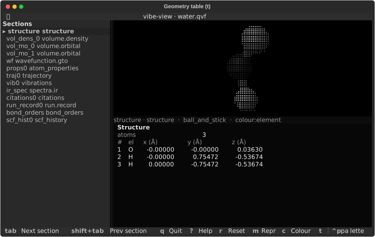
t opens the data table for the current section. On a structure that is the geometry: cell parameters when periodic, Cartesian coordinates, and the bond list with orders and lengths.

What each section kind shows

Drawn in 3-D: structure, trajectory, reaction.path, vibrations, every volume.*, basis.ao, and wavefunction.gto in the TUI. Volumes draw their isosurface over the structure; signed fields get both lobes, unsigned density one surface. Trajectories and reaction paths also have an energy-profile chart (g in the TUI, --chart for show).

Charted: bands, dos.total, dos.projected, dos.coop, dos.cohp, every spectra.* stick spectrum, scf_history, equation_of_state, phonon_bands, phonon_dos, and scan.surface as a colour heat map. The conventions match the browser’s Plotly charts so the two tell the same story: bands and DOS are Fermi-referenced when E_F falls inside the data window and labelled absolute when it does not; SCF convergence is |ΔE| on a log axis; spectrum axes carry each kind’s native unit, with the Lorentzian envelope named in the legend.

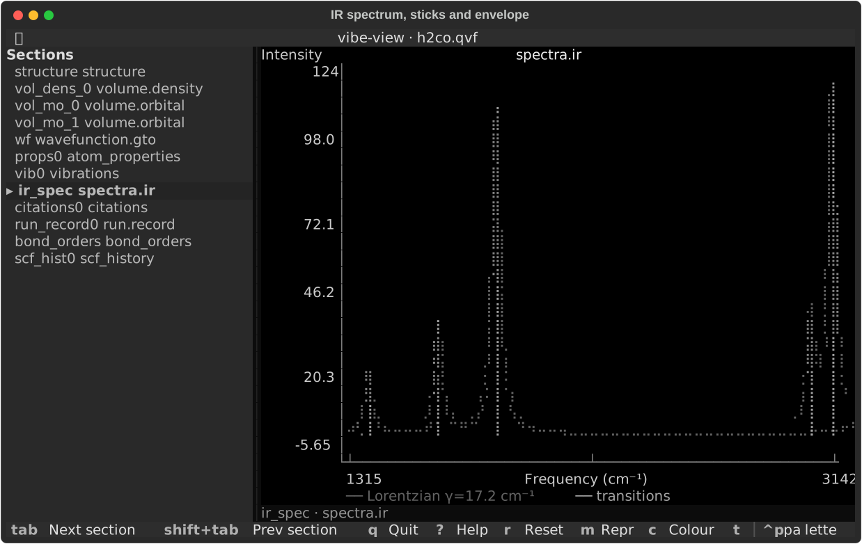
An IR spectrum: the computed transitions as sticks, the envelope drawn under them and named, so the convenience is never mistaken for the data.

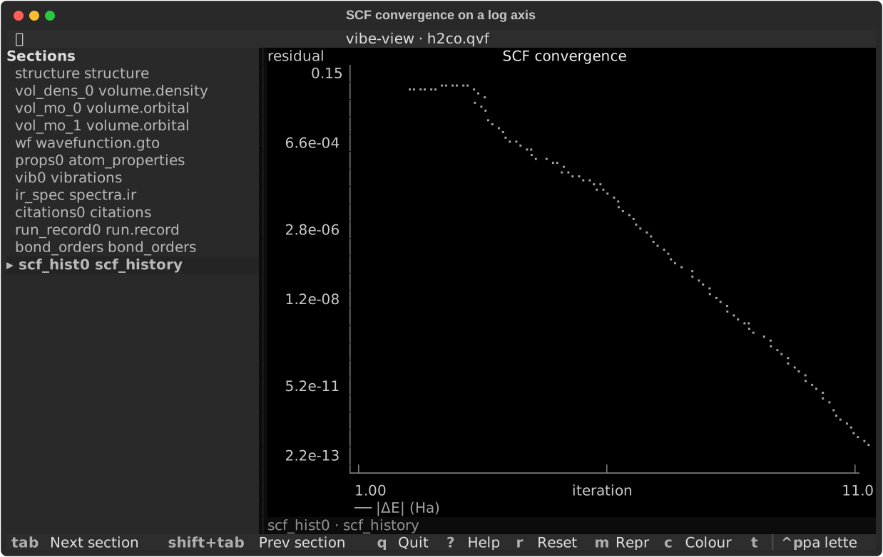
SCF convergence, |ΔE| on a log axis.

Tabulated: citations (BibTeX ready to paste), run.record (the invocation, its verbatim input and the tail of its log), job.spec, atom_properties, bond_orders, structure.symmetry, spectra.nmr, spectra.epr, topology.qtaim.

Any kind the viewer does not draw still appears in the browser with the reason from the kind registry: not yet rendered is a different statement from unsupported.

Orbitals on demand

Activating a wavefunction.gto section evaluates a default orbital, the frontier orbital when one is well defined, and opens a focusable surface table on the right.

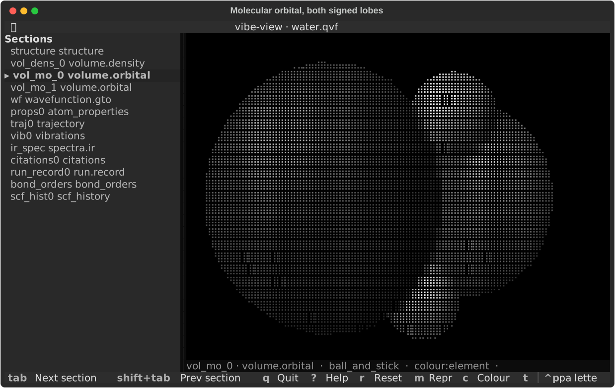
A molecular orbital in the TUI, evaluated from the basis and the coefficients rather than read from a stored grid.

1. ↑ / ↓ highlight a row; Enter or a mouse click renders it.

2. n / p step through orbitals directly.

3. i / I lower or raise the contour; o hides it.

4. Total density (D) is the first row when the archive declares electron-occupation semantics. A natural-transition-orbital set declares transition weights instead, so the row is absent and the key explains the refusal; a legacy natural set without either declaration renders its orbitals but not a guessed density.

5. Spin density α − β (S) exists for an unrestricted wavefunction and is refused, with a reason, for a restricted one.

Every wavefunction set in the archive, canonical, alpha/beta, natural or localized, gets its own table and remembered selection. Canonical rows are identified by energy and occupation, natural rows by occupation or transition weight, localized rows by the atoms they sit on, because a localized orbital has no meaningful energy ordering. The status line always names the rendered row, its spin and the isovalue.

Sampling uses a terminal-sized 48³ grid; the first render of a large basis takes a moment, and stepping back to a sampled row uses the cache. The evaluator covers shells through l = 3 and marks a surface incomplete when an orbital has significant g-or-higher weight. Periodic wavefunctions are Gamma-point fields from central-cell atomic orbitals; image tails are not added.

Biomolecules

An all-atom render of a solvated protein is a solid mass at terminal resolution. Use the backbone trace instead:

vibe-view show protein.qvf --representation backbone
vibe-view show protein.qvf --color-by chain
vibe-view show protein.qvf --color-by bfactor

backbone draws one point per alpha carbon, joined along each chain and coloured by secondary structure: red helix, yellow strand, grey coil. Chains are traced separately, so no bond is ever drawn from one chain’s C-terminus to the next chain’s N-terminus. bfactor ramps blue to red across the temperature factors and falls back to element colouring when the column carries no variation, which is common; the status line says which scheme is actually shown and why. See Biomolecules for how the metadata gets into the file.

Rendering modes

braille (default) packs a 2×4 dot matrix into every character cell: eight times the geometric detail of block characters, at the cost of one colour per cell, the average of what the eight dots cover. Best for structures and isosurfaces, where shape carries the meaning.

half (--mode half, d in the TUI) splits each cell into two independently coloured pixels. A quarter of the vertical resolution, but two true colours per cell: better for heat maps and anything where colour is the data.

Consistency with the other surfaces

Element colours and radii come from the same functions the browser viewer and every PNG capture use, including any per-element override you have set in the browser’s settings, so a terminal frame and a screenshot of the same archive agree on what carbon looks like. Periodic systems follow the same rules as the 3-D renderer: cell edges only along periodic axes, and bonds across a cell face drawn to the nearest periodic image rather than stretched across the box.

That last rule matters more than it sounds. A periodic bond list stores the in-cell index pair, so graphene’s 1.42 Å bonds are listed at separations of 2.84, 3.76 and 5.68 Å. Drawing those endpoints literally produces a hairball; filtering by length deletes real bonds.

From Python

render_terminal is on the public SDK, next to the PNG capture functions: the same renderers, a string instead of an image, and no GL context.

from vibeview import render_terminal

print(render_terminal("job.qvf", size=(100, 30)))
print(render_terminal("job.qvf", "vol_mo_3", isovalue=0.03))

# plain=True drops the ANSI colour, for a log file
open("frame.txt", "w").write(render_terminal("job.qvf", plain=True))

It accepts a path, a file-like object or an already-open QVFReader, and a reader you pass in stays open. Keyword arguments match the show flags: mode, representation, color_mode, replication, isovalue, rotation, show_labels, frame, chart. A section with no graphical form returns a short explanation rather than raising, so sweeping every section needs no pre-filtering by kind.

The layers underneath are importable for finer control: vibeview.tui.show.render_section returns the cell grid before it is stringified, vibeview.tui.plots builds charts, vibeview.tui.panes the text panes, and vibeview.tui.scene with vibeview.tui.raster are the scene builder and the rasterizer.

A runnable script covering all of it ships in the checkout:

python examples/terminal_mode.py job.qvf
python examples/terminal_mode.py job.qvf --plain

It branches on what the archive actually contains, so it is safe to point at any .qvf.

Limits

• No mouse rotation. Use the keys.

• One colour per braille cell, so two differently coloured atoms sharing a cell blend. Zoom in, or use --mode half.

• Large volumes contour on every isovalue change. A 100³ grid is quick; a 300³ grid takes a moment.

• The text panes are read-only, except the wavefunction surface table. Use vibe-view export and vibe-view table to get data out.

It is a reading tool: fast, low-resolution, no setup, works over SSH. For publication figures use vibe-view capture or the browser’s own export; for a native window, the desktop app.