A tour of the viewer
You will learn: what each panel of the browser viewer shows, using an archive that carries the full set of section kinds, and how the same archive looks in the terminal and from Python.
You need: an installed vibe-view with the default modes profile, and a
.qvf file with something in it. The bundled demo carries a single
structure section, which is enough for the first two stops; the rest of
the tour needs sections from a producer. The figures use computed
vibe-qc showcase archives, with explicitly
illustrative fixtures for panels that the available archives do not carry.
These are captures of the actual viewer, not generated artwork. The
regeneration notes record the inputs.
Time: about ten minutes.
1. Something to look at
vibe-view demo -o water.qvf          # a structure-only archive, no producer needed
vibe-view info water.qvf             # what is in it
If you have your own archive, use that instead, and ask it the same question first:
vibe-view info calculation.qvf
info lists every section with its kind and size. Anything listed here gets
a sidebar entry; anything not listed is not in the file, however hard you
look for it in the viewer.
2. Open it
vibe-view open calculation.qvf
The terminal prints the startup banner, one row per section with its render
status, and your browser opens at http://127.0.0.1:8080. The server stays
in the foreground until you press Ctrl+C.
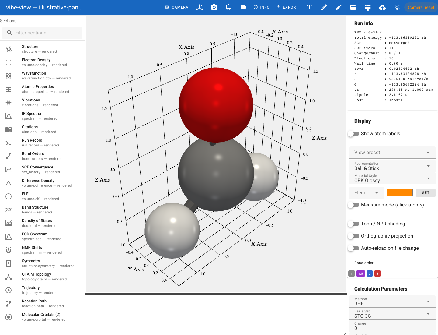
The structure panel. Sidebar on the left, viewport in the centre, the section’s controls on the right.
Rotate with a left drag, pan with a middle drag, zoom with the wheel, r to reset. Press ? for the shortcut list and Ctrl/Cmd+K for the command palette, which also jumps to any section by name.
3. The structure
The first section to activate is the structure: CPK-coloured atoms, bonds from the file’s own connectivity or inferred from covalent radii. Try the Representation picker in the Display card, then a Material Style. Switch on Show atom labels, then press m and click two atoms for a distance, a third for the angle.
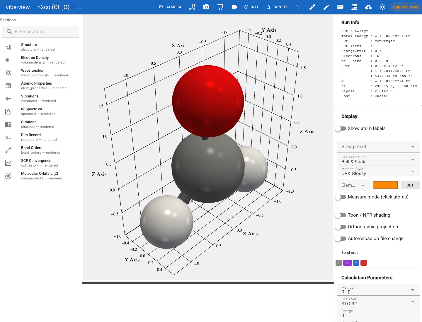
Formaldehyde in ball-and-stick.
4. Density and difference density
Click a volume.density section. The payload is read from the archive now,
not at open time, and the isosurface appears translucent over the structure
at the default isovalue of 0.05 e/bohr³. Drag Volume isovalue down and
the surface grows outward; drag it up and it collapses onto the nuclei. The
lone-pair region is where the density stays largest as you raise the
isovalue.
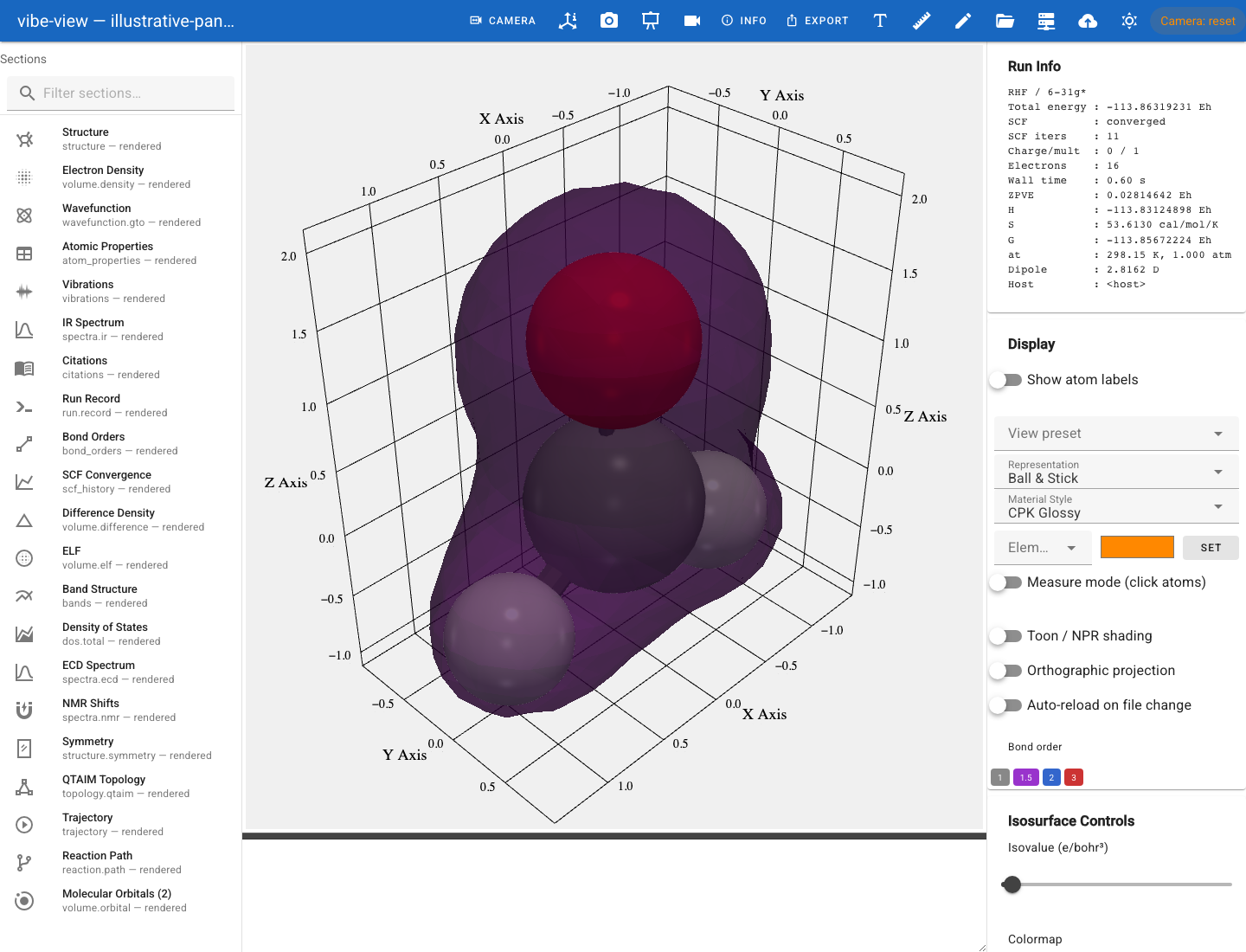
The electron density.
A volume.difference section is a signed field and draws both signs at
once: where density accumulated and where it left.
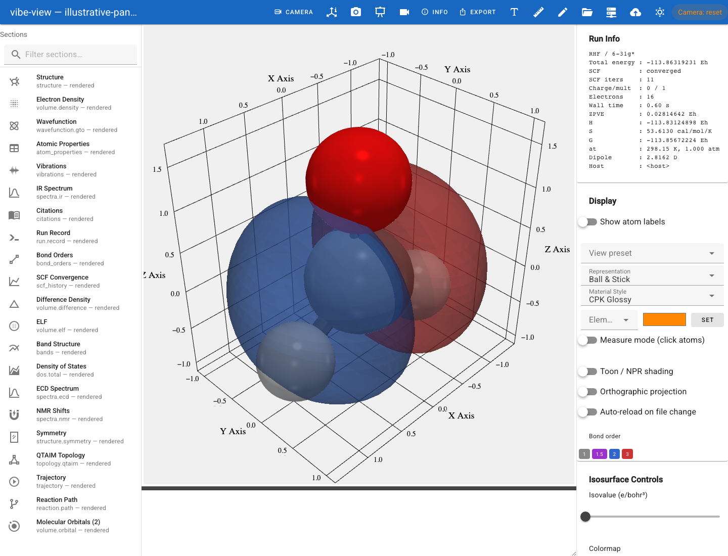
A difference density. This capture uses illustrative panel data.
5. Orbitals: stored and on demand
A volume.orbital section is an orbital the producer pre-evaluated on a
grid. It renders like any other signed field, with both lobes in contrasting
colours.
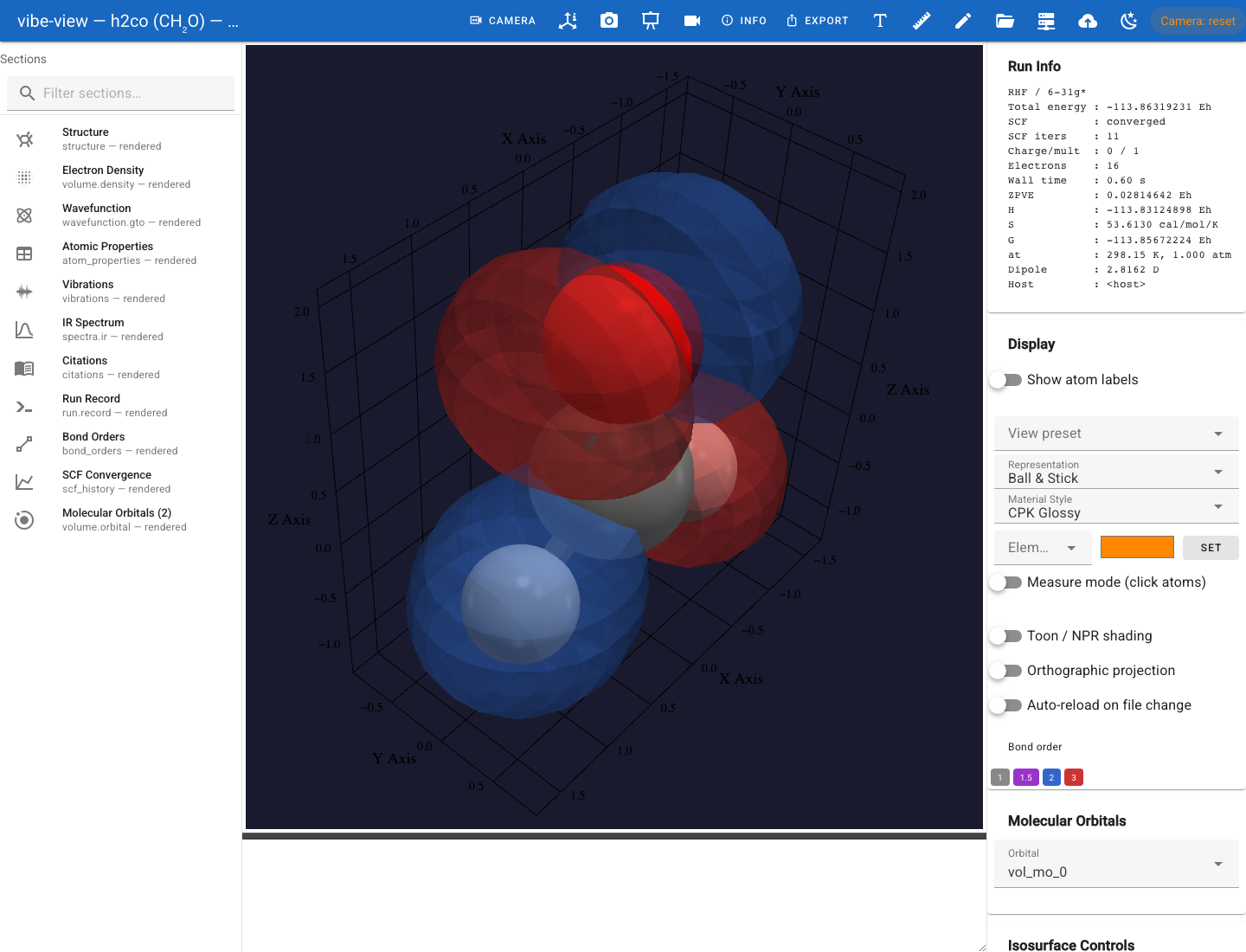
A stored orbital grid.
A wavefunction.gto section is different, and better: it carries the basis
and the coefficient matrix, and the Molecular Orbitals panel evaluates
whichever orbital you click. Press the HOMO button, then the next-orbital
arrow a few times. Nothing was pre-computed; each surface is sampled when you
ask for it, and cached after that.
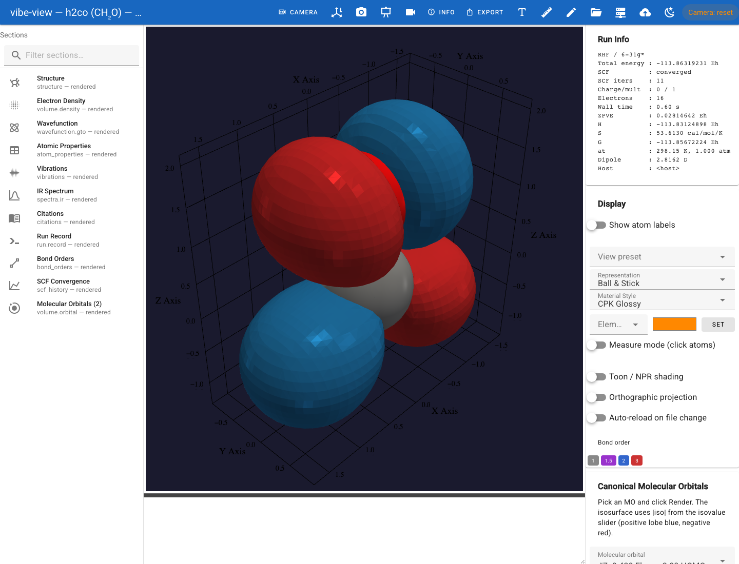
The HOMO, evaluated on demand.
Compute total density sums the occupied orbitals and reports the integrated electron count, a quick sanity check that the wavefunction in the file is the one the producer meant to write.
6. Charges
atom_properties becomes the Population Analysis table, and Color
atoms by charge paints the result onto the atoms, red positive and blue
negative.
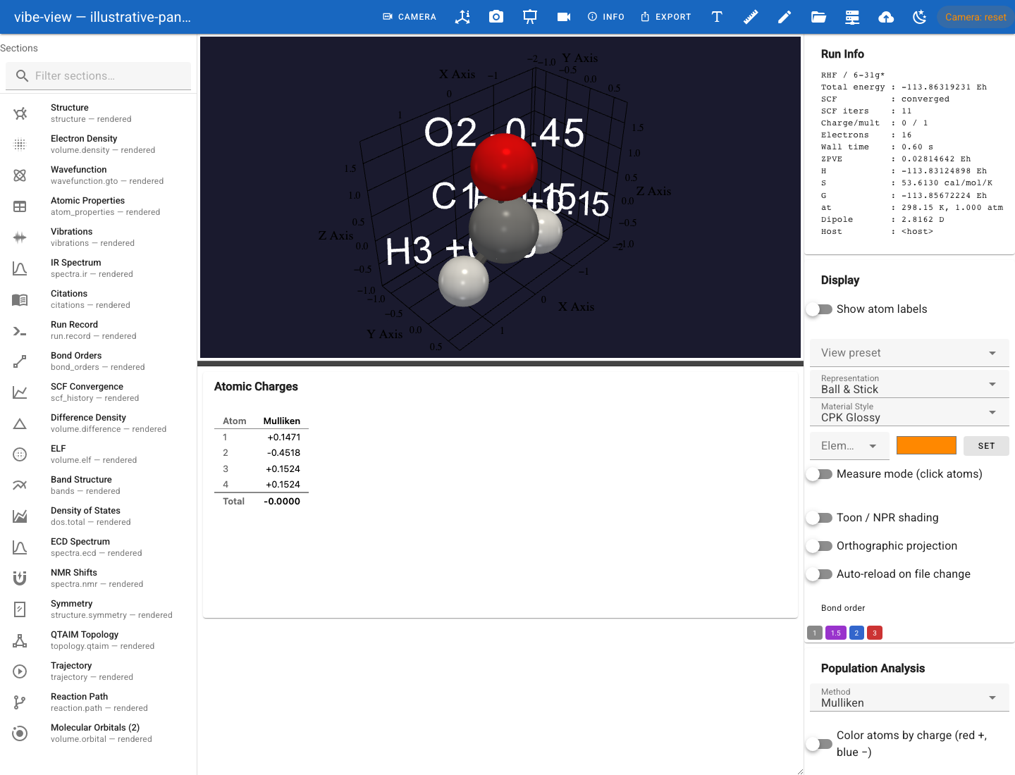
Charges as a table and as an overlay.
7. Vibrations and the IR spectrum
Click vibrations, then a mode in the list. The structure oscillates along
that mode’s displacement; Vibration displacement amplitude exaggerates
it. With a companion spectra.ir section the mode labels carry the IR
intensity, and the spectrum itself is a stem chart with hover tooltips.
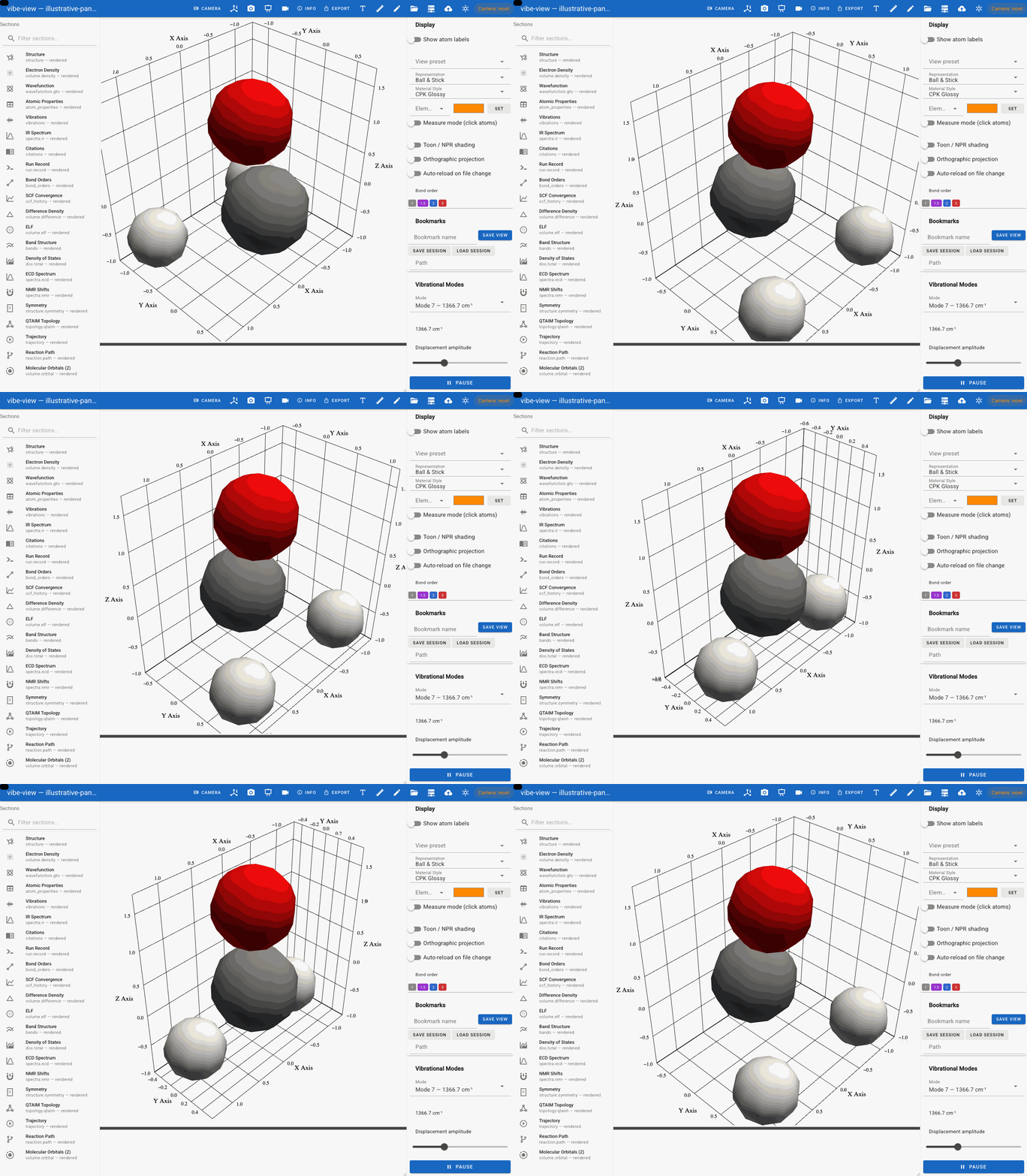
A normal mode.
8. Trajectories and reaction paths
A trajectory section is an optimisation, frame by frame, with the energy
profile tracking the current frame. A reaction.path adds the waypoints:
reactant, transition state, product.
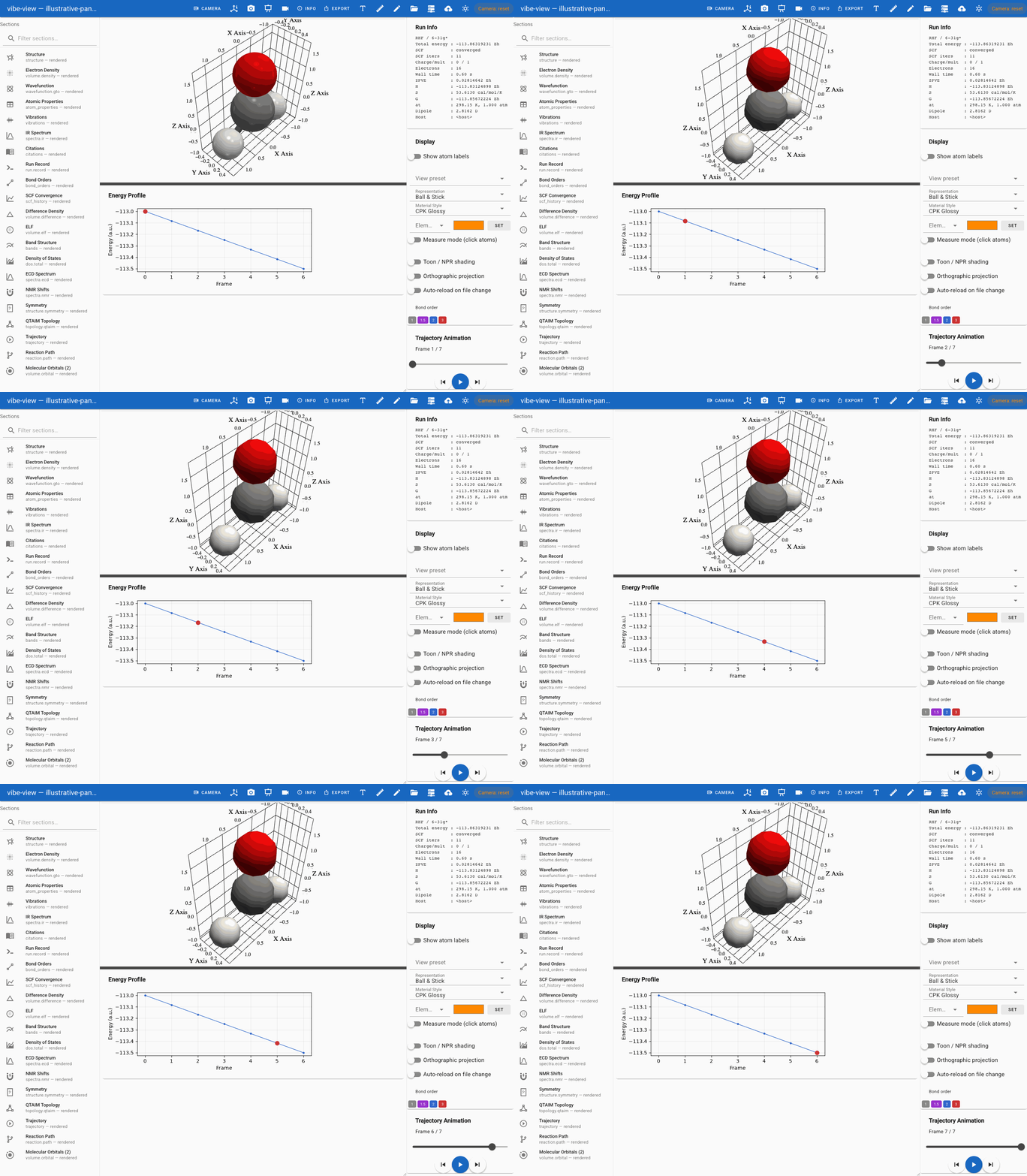
An optimisation trajectory. This capture uses illustrative panel data.
9. Convergence and provenance
scf_history plots the energy and the DIIS error per iteration.
citations is the BibTeX bundle the producer says this calculation should
cite, ready to paste. run.record, when present, is the executed input and
the log.
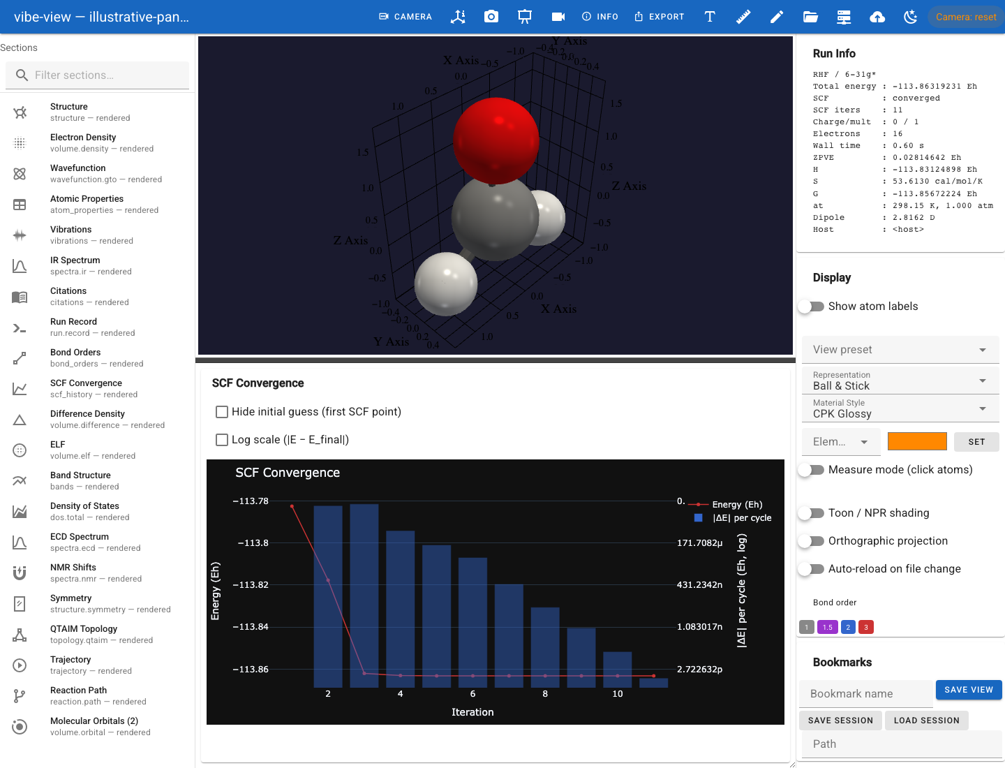
SCF convergence.
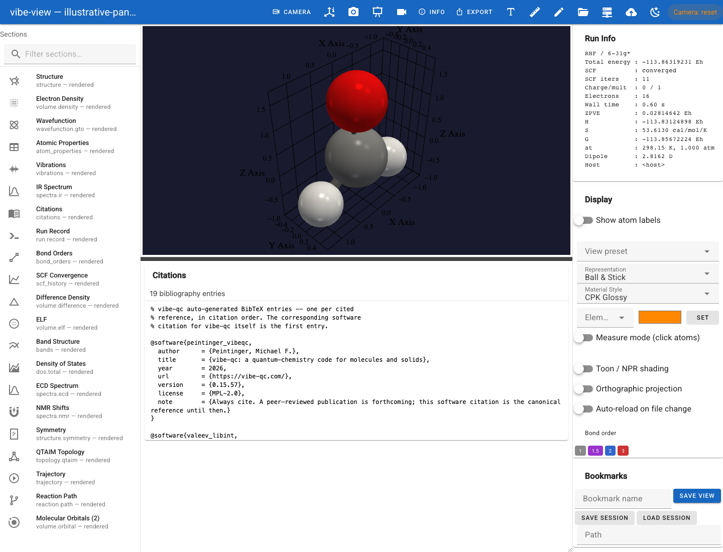
The citations panel.
10. A periodic file
Open a periodic archive and the structure panel gains a unit-cell wireframe
and the Periodic Replication controls. Set Nx = Ny = Nz = 2 and the
atoms, the cell, the bonds and any active isosurface tile together.
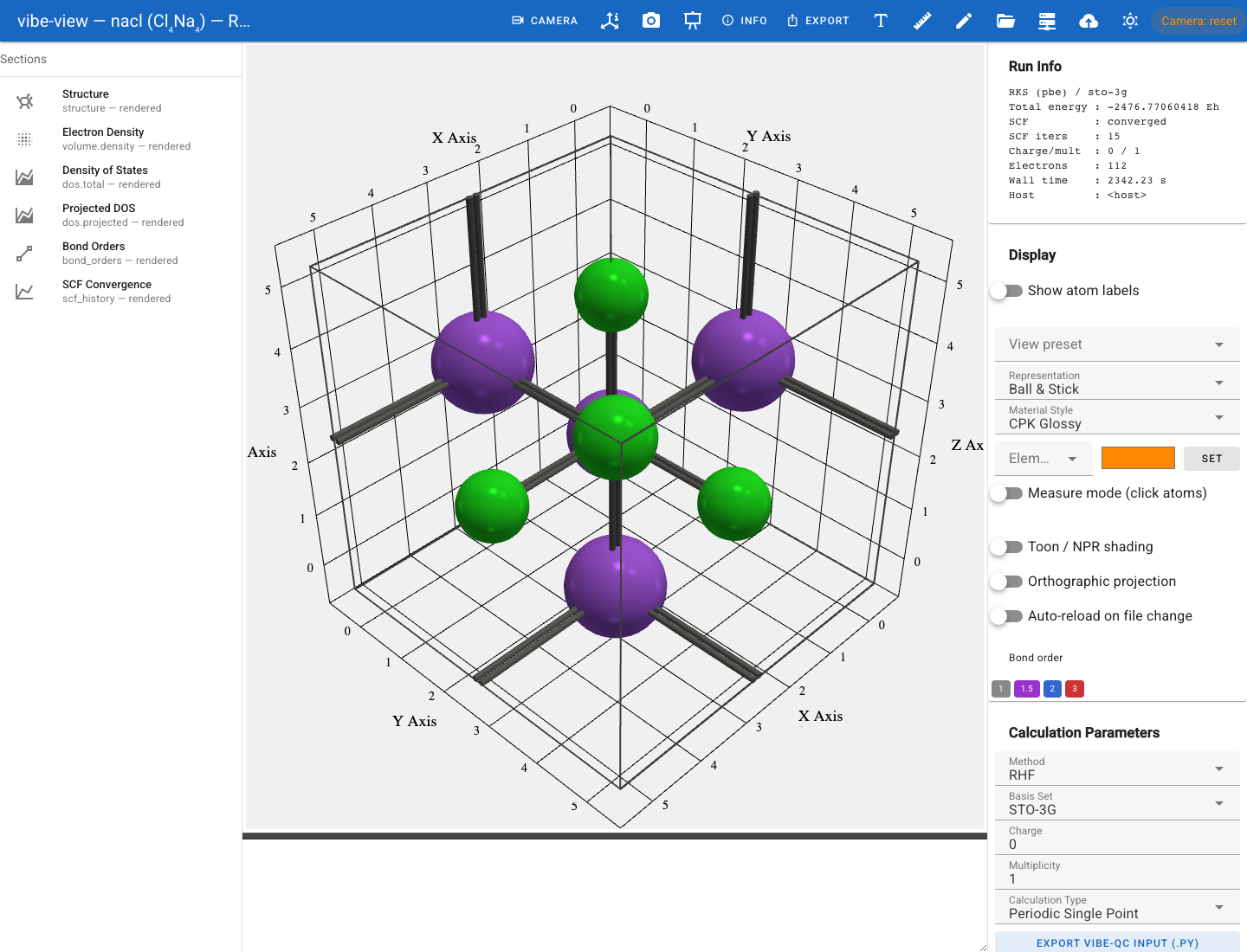
A crystal, replicated.
bands and dos.total are drawn as one figure on a shared,
Fermi-referenced energy axis.
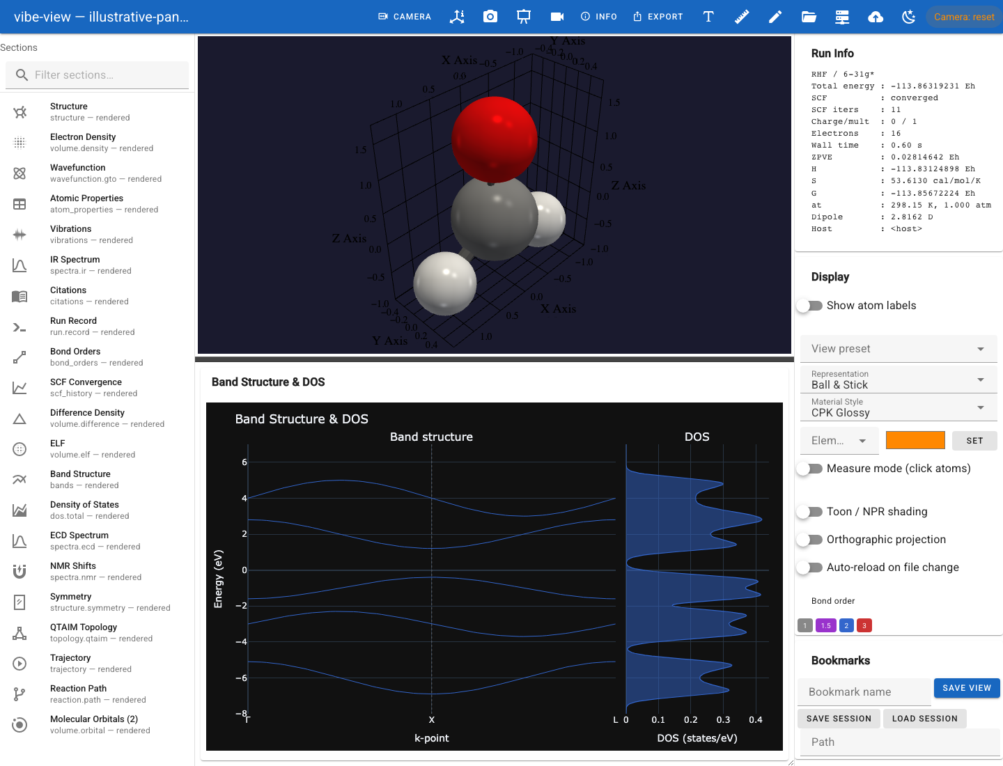
Band structure and density of states. This capture uses illustrative panel data.
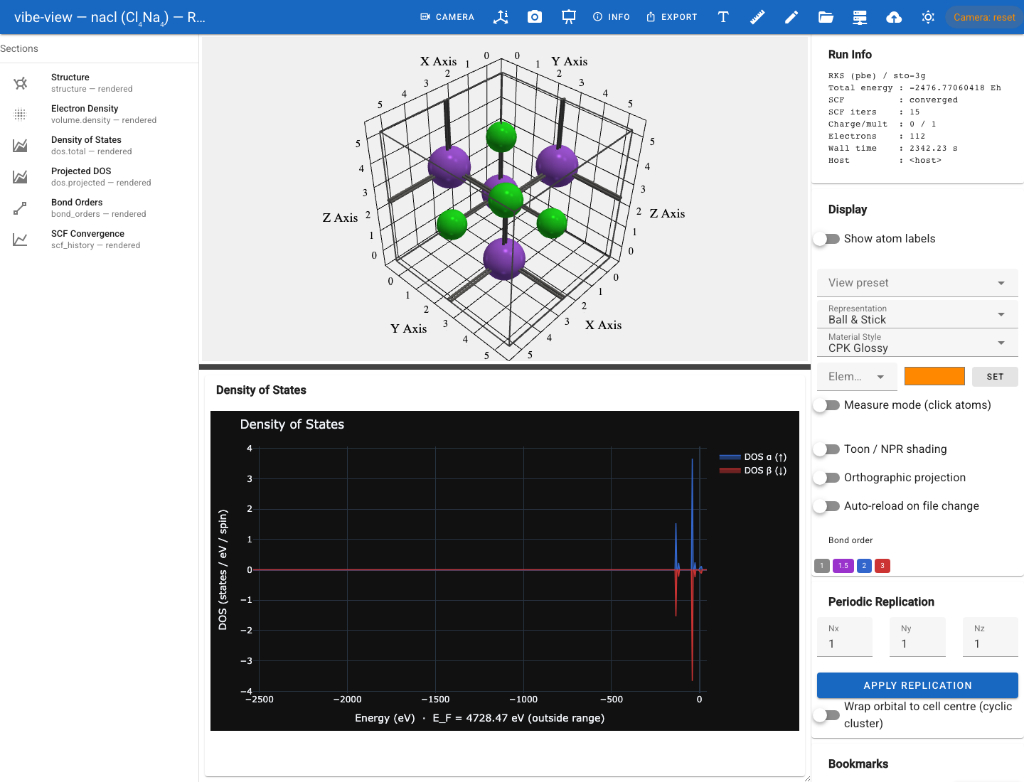
The density of states on its own: valence band below the gap, conduction band above.
11. Two files at once
vibe-view compare a.qvf b.qvf
Both structures appear overlaid, one translucent colour per file, with a legend. Switch on Align (RMSD fit to first file) and the second is Kabsch-superposed onto the first with the RMSD shown, so the displacement you see is the geometric difference rather than a difference in coordinate frame. If both files carry a density on the same grid, the Density Difference card draws ρ_A − ρ_B as a two-colour surface.
12. Save the views you found
Set up a view, type a name in the Bookmarks card and press Save View. Do it for the structure, the density and the HOMO, then Save Session. Next time, Load Session brings every bookmark back, and p turns them into a slideshow.
13. The same archive, elsewhere
Everything above came out of one file, and the file does not care which surface reads it:
vibe-view show calculation.qvf                     # one braille frame, no display needed
vibe-view show calculation.qvf -s homo --isovalue 0.03
vibe-view tui calculation.qvf                      # the interactive terminal viewer
vibe-view capture calculation.qvf -s density -o density.png
vibe-view desktop calculation.qvf                  # a native window
from vibeview import QVFReader, get_table

with QVFReader("calculation.qvf") as r:
    for s in r.sections:
        print(s.id, s.kind)
headers, rows = get_table("calculation.qvf", "atom_properties")
Where next
The browser viewer, the reference for every control on this tour.
Building and editing, for changing the structure rather than looking at it.
Terminal mode, for the compute node.
Figures without a display, for the paper.