Worked example: Raman and VCD through ORCA and vq

This example uses one twisted hydrogen-peroxide conformer to exercise IR, Raman and signed VCD spectra together. The supplied results were calculated with ORCA 6.1.1 through vq, using PBE/def2-SVP and analytical frequencies. A reflected geometry provides an independent check of the VCD sign.

The tutorial also closes the loop from a calculated vibration to a new calculation: combine selected modes, export the edited geometry, then submit and inspect a new ORCA single point. That follow-up has its own result archive and browser screenshots.

Dataset	What was calculated	Download
Original peroxide	Optimization, normal modes, IR, Raman and VCD	peroxide.qvf
Reflected peroxide	Frequencies, Raman and opposite-sign VCD	mirror.qvf
Combined-mode displaced peroxide	Single-point energy, orbitals, charges and bond orders	peroxide-displaced-sp.qvf

Open each archive separately to keep its geometry and calculated properties together. The original modes define the displacement; the follow-up archive contains the electronic properties calculated at the new coordinates.

1. Get the example

Download these files into a new directory:

• Starting geometry.

• Optimization and spectroscopy input.

• Native calculated Hessian.

• Scientific VCD output excerpt — final geometry, printed table and completion marker from the real run, with operational details omitted.

• Complete viewer dataset.

To inspect the supplied results without installing ORCA or vq:

vibe-view open peroxide.qvf

For a new calculation, follow ORCA and vq setup. Raman analytical derivatives in this workflow require ORCA 6.1 or newer. VCD requires analytical frequencies and is unavailable with NumFreq. The FACCTs vibrational spectroscopy chapter describes both calculations and the meaning of Raman activity.

2. Prepare and submit

Open peroxide.xyz, select Structure, and open Calculation Parameters. Choose ORCA, PBE, def2-SVP, charge 0, multiplicity 1, one process, and 1000 MB MaxCore. Choose Single Point + Freq + Opt and enable Raman activities (ORCA 6.1+) and VCD rotatory strengths. Preview the input: it includes Opt AnFreq, %elprop Polar 1 end and %freq doVCD true end. Save a copy, then use Submit ORCA to vq and Fetch & open results, as in the water tutorial.

For the exact reference run, use the downloaded input below. It tightens the optimization with TightOpt; the basic form uses Opt. Downloaded-file edits do not change what the viewer form submits. Submit the edited input directory through the vq command line:

! PBE def2-SVP TightSCF TightOpt AnFreq
%pal nprocs 1 end
%maxcore 1000
%elprop Polar 1 end
%freq doVCD true end
* xyz 0 1
O -0.725 0.000 0.000
O  0.725 0.000 0.000
H -1.020 0.920 0.000
H  1.020 -0.300 0.870
*

mkdir peroxide-run
cp calculation.inp peroxide-run/
vq submit localhost -d peroxide-run --program orca --cpus 1 --mem-mb 1334 \
  --wall-time-seconds 600 --job-name orca-peroxide -- /opt/orca/orca calculation.inp

Replace /opt/orca/orca with your installed executable. Use the job identifier returned by your submission:

vq status localhost JOB_ID
vq logs localhost JOB_ID
vq fetch localhost JOB_ID -o fetched

Wait for completion and ORCA TERMINATED NORMALLY. In the fetched job directory, keep calculation.property.txt, calculation.gbw and calculation.hess together, including vq’s stdout.log for VCD. Set up the matching orca_2json, then run:

vibe-view open calculation.hess

The viewer combines the structure, orbitals, properties, vibrations and all three vibrational spectra. A standalone Hessian opens its geometry, modes and IR/Raman spectra without an ORCA installation. VCD comes from the matching completed output log; ORCA 6.1.1 does not write it to the Hessian or property file. The downloadable output excerpt can be paired with the supplied Hessian to exercise this import without GBW.

3. Inspect Raman and VCD

1. Select Vibrations to inspect the optimized structure and animate a mode. ORCA numbers modes from zero; the viewer’s mode selector starts from one.

2. Select Raman Spectrum. Set Display to Sticks only and leave Normalize off. The vertical axis is scattering activity in Å⁴/amu. The imported JSON also retains each mode’s depolarization ratio.

3. Select VCD Spectrum, again with normalization off. Positive and negative sticks must remain on opposite sides of zero. Read the rotatory-strength unit on the axis; these values are not molar Δε.

4. Switch to Envelope + sticks to inspect overlapping bands. Changing broadening changes the displayed curve, not the stored strengths. No laser-frequency, temperature or experimental-intensity correction is applied to Raman activities.

5. Select Wavefunction for the orbitals or Atomic Properties for the final-geometry charges. They belong to this same calculation dataset.

Drag the divider above Result details upward to enlarge the chart.

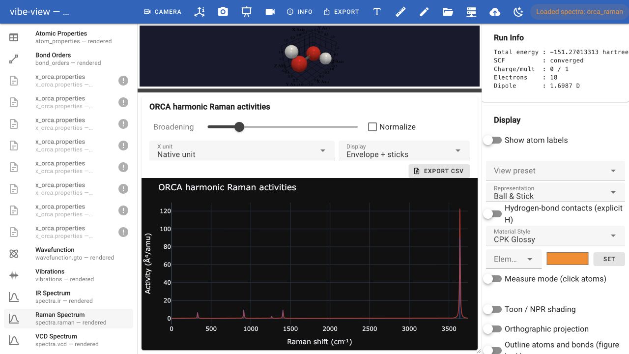
Raman activities from the fetched Hessian. The broadened curve sums nearby bands; switch to sticks when comparing the tabulated activities.

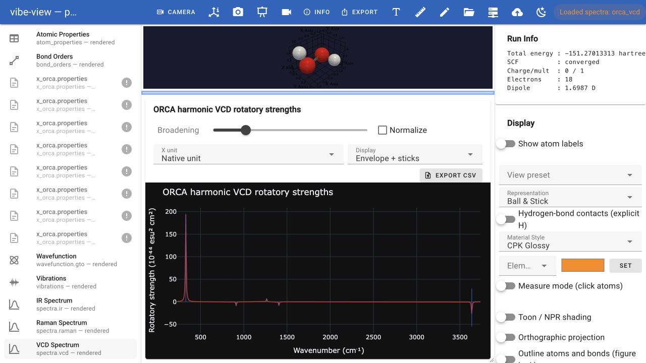
The completed output’s VCD strengths, with their signs and native units.

Prepare two structures along a mode

Use the peroxide result above to prepare two starting geometries:

1. Select Vibrations, then the mode near 328.825 cm⁻¹. In this full Hessian, it is viewer Mode 7, corresponding to ORCA index 6.

2. Below the animation controls, set Signed peak displacement (Å) to 0.10 and click Create displaced structure. The viewer opens Structure → Atom Editor and stops animation and auto-optimisation.

3. Click Save geometry (XYZ) and save it as peroxide-mode6-plus.xyz. The largest atomic shift is 0.10 Å from equilibrium; the remaining shifts follow the relative lengths and directions of the mode vectors.

4. Return to Vibrations, choose the same mode, set the signed value to −0.10, and click Create displaced structure again. Save it as peroxide-mode6-minus.xyz. This starts from equilibrium again, so the positive and negative offsets are equal and opposite. Undo returns to the positive geometry.

5. For either geometry, select Calculation engine → ORCA, choose the method, basis, charge 0, multiplicity 1 and calculation type you want, then Preview ORCA input and Save ORCA input (.inp). Follow the submission steps to send the edited structure through vq into a new job.

The archived result remains unchanged. The displayed spectra, frequencies and orbitals belong to that original calculation, not to either displaced geometry. These steps prepare new inputs; they do not claim that the new jobs have run or that the displacement leads to a different minimum. For an imaginary mode in another calculation, the same controls produce starting geometries on either side of its stored direction. See the editing guide for limits and the full-mode/frozen-atom behavior.

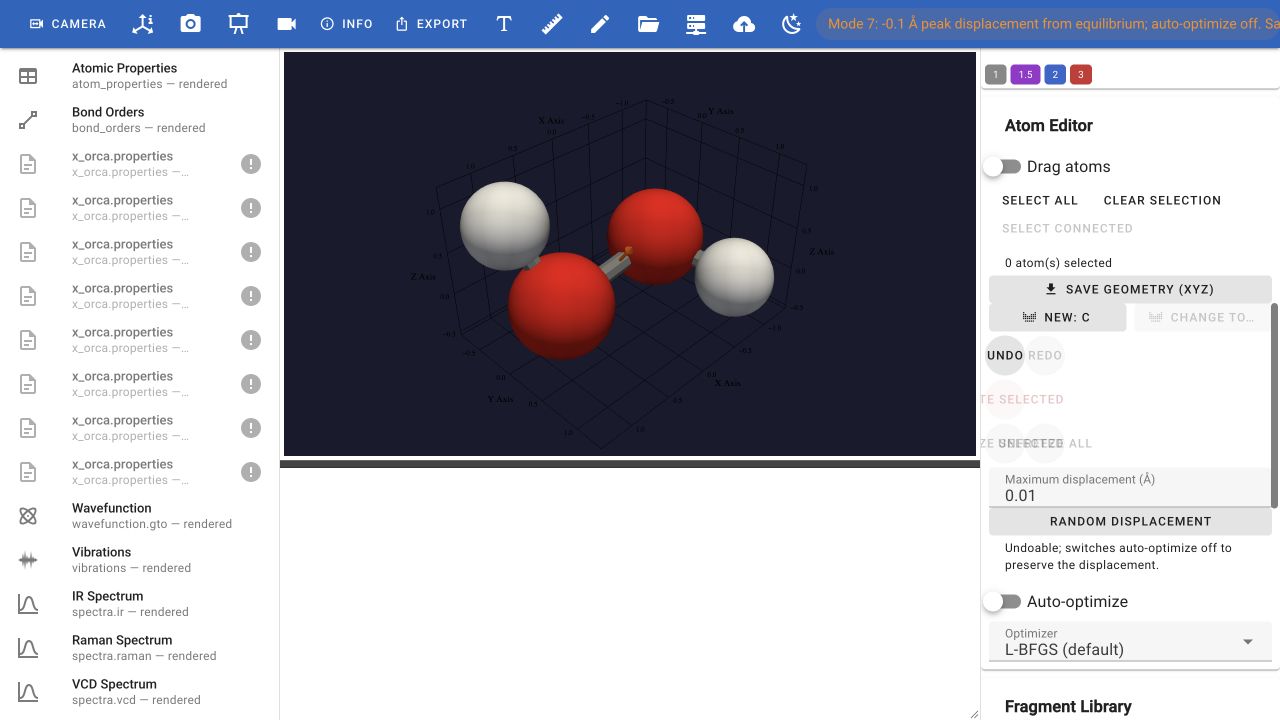
The real peroxide result after creating the negative displacement. The status bar identifies the mode and sign; the geometry is ready for export.

Combine selected modes

This walkthrough uses the supplied peroxide.qvf; no new ORCA calculation is needed to try the displacement. Start from a freshly opened archive so that Undo returns to its equilibrium geometry.

1. Select Vibrations and expand Modes to displace below the animation controls. Select Mode 7 — 328.8 cm⁻¹ and Mode 8 — 911.4 cm⁻¹, then close the selection menu. These are ORCA indices 6 and 7.

2. Set Mode 7 signed peak displacement (Å) to 0.10 and Mode 8 signed peak displacement (Å) to −0.05. Leave each field after typing so its value is applied. The separate animation selector and animation amplitude do not set these geometry edits.

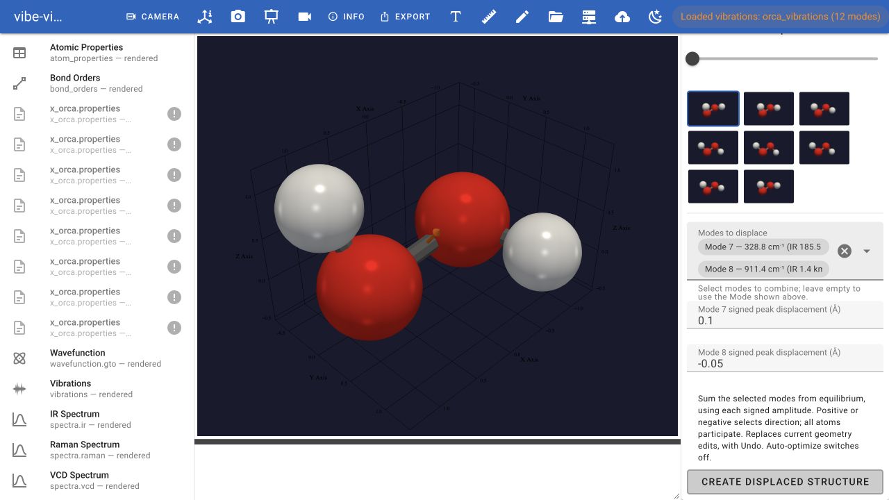
Select both modes and give each its own signed displacement. The central view at this stage previews the animation mode, not the combined edit.

3. Click Create displaced structure. The viewer opens Structure → Atom Editor, stops animation, and switches auto-optimisation off. The status identifies both modes and amplitudes, summed from equilibrium.

4. Click Save geometry (XYZ). In a local browser session this writes a timestamped XYZ beside the opened file as well as offering a download. If no download appears, check that directory. Rename your copy if desired. Compare it with the reference combined XYZ.

5. In Calculation Parameters, select ORCA, PBE, def2-SVP, charge 0, multiplicity 1, and Single Point. Click Preview ORCA input. Its Cartesian block must use the displaced coordinates. The reference input was captured from this browser preview.

6. Click Undo, then Preview ORCA input again to refresh the text: the equilibrium coordinates return. Click Redo and preview again: the combined coordinates return. Save the input with Save ORCA input (.inp) when satisfied. To calculate it, follow the ORCA submission steps and use a new job directory through vq.

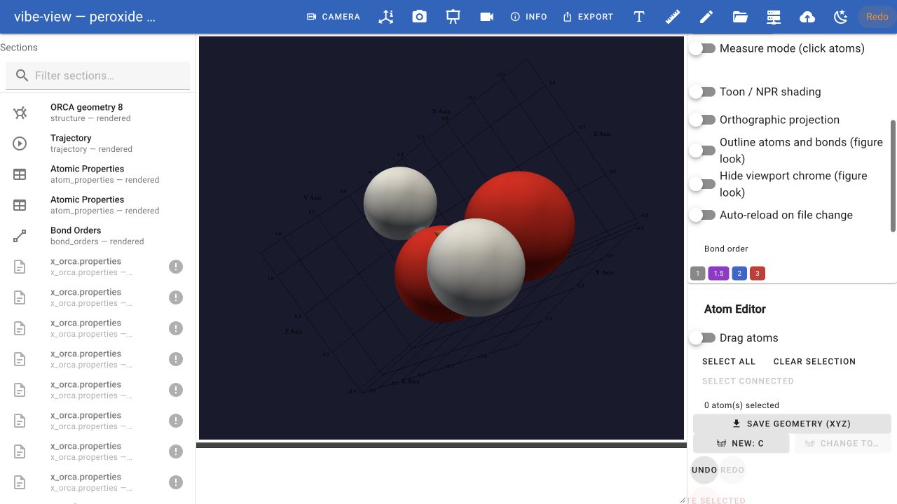
The combined structure after Undo and Redo. Save geometry exports this edit; the original calculated dataset remains available in the section list.

Each mode is scaled independently so its largest atomic displacement has the requested magnitude. The viewer then adds the signed contributions: R = R_eq + 0.10 d_6 / max_i|d_6,i| − 0.05 d_7 / max_i|d_7,i|. It does not renormalize the sum. Consequently, the largest combined atomic shift in this example is 0.08454913 Å, not 0.10 or 0.15 Å.

These steps were checked in the browser against source revision 51113e7. An independent sum of the archived vectors matched every coordinate in the ORCA preview within 5 × 10⁻¹¹ Å, and the six-decimal XYZ export within 5 × 10⁻⁷ Å. Undo restored equilibrium to preview precision; Redo reproduced the original combined preview exactly. These tolerances describe text rounding, not the accuracy of the electronic-structure calculation.

The downloadable combined files are prepared starting geometries, not new calculated results or an IRC path. The spectra, frequencies, orbitals and energies in the open archive still belong to the original equilibrium calculation. The next walkthrough calculates the exported combined geometry and opens its results as a separate dataset.

Calculate the displaced structure through vq

This follow-up was run with ORCA 6.1.1 through vq and inspected in the browser. It uses exactly the combined-mode input above: PBE/def2-SVP, TightSCF, one process and a single point. Download the calculated dataset to inspect the result immediately, or repeat the full workflow below. The scientific output excerpts provide the numerical reference; they are not the complete restart files.

1. After applying the selected modes (or Redo after an Undo check), use Preview ORCA input → Save ORCA input, or download the reference peroxide-selected-modes.inp. Put only this input into a fresh job directory:

   mkdir peroxide-displaced-run
   cp peroxide-selected-modes.inp peroxide-displaced-run/calculation.inp
   

2. Submit that directory through vq. This example uses a configured local queue; substitute your queue host and the absolute ORCA executable path on that host. The input requests %maxcore 1000; the queue reservation below includes additional memory headroom.

   vq submit localhost -d peroxide-displaced-run --program orca \
     --cpus 1 --mem-mb 1334 --wall-time-seconds 600 \
     --job-name orca-peroxide-displaced -- /opt/orca/orca calculation.inp
   

3. Copy the returned job ID into JOB_ID. Check the queue state and output, then fetch the completed job:

   JOB_ID=replace-with-returned-job-id
   vq status localhost "$JOB_ID"
   vq logs localhost "$JOB_ID" --stdout
   vq fetch localhost "$JOB_ID" -o fetched
   

   The reference job reached completed, exit code 0, and ORCA TERMINATED NORMALLY. Acceptance into the queue alone does not establish completion. Use the result directory printed by vq fetch; its name includes the job name and ID.

4. In that fetched directory, keep calculation.gbw, calculation.property.txt and stdout.log together. Import the GBW with the matching ORCA 6.1.1 orca_2json utility, then validate and open:

   cd "fetched/orca-peroxide-displaced-${JOB_ID}"
   export ORCA_2JSON=/opt/orca/orca_2json
   vibe-view import calculation.gbw -o peroxide-displaced-sp.qvf
   vibe-view validate peroxide-displaced-sp.qvf
   vibe-view open peroxide-displaced-sp.qvf
   

   The importer runs the utility and combines the companion properties into one dataset. The reference archive validates with 6 sections and 8 members. Opening the downloaded QVF needs no ORCA installation.

5. Select ORCA geometry 1. Run Info shows a converged SCF, charge 0, multiplicity 1, 18 electrons, energy −151.26444845 hartree and dipole 1.9381 D. The four imported atomic positions agree with the submitted Cartesian input within 5 × 10⁻⁹ Å. This is the displaced geometry, not a newly optimized minimum.

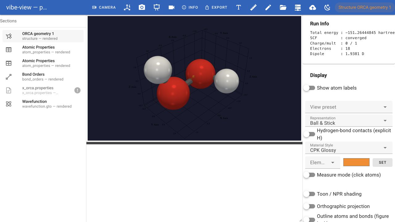
The fetched single-point result opened as one dataset in vibe-view.

6. Select Wavefunction and click HOMO, then LUMO. Both render directly from the imported coefficients. This restricted calculation contains 38 spatial orbitals, of which 9 have occupation 2. ORCA’s zero-based HOMO index is 8 (−0.200234 Eh), and the LUMO index is 9 (+0.027409 Eh). The screenshot uses 60 grid points per axis and an orbital isovalue of 0.05.

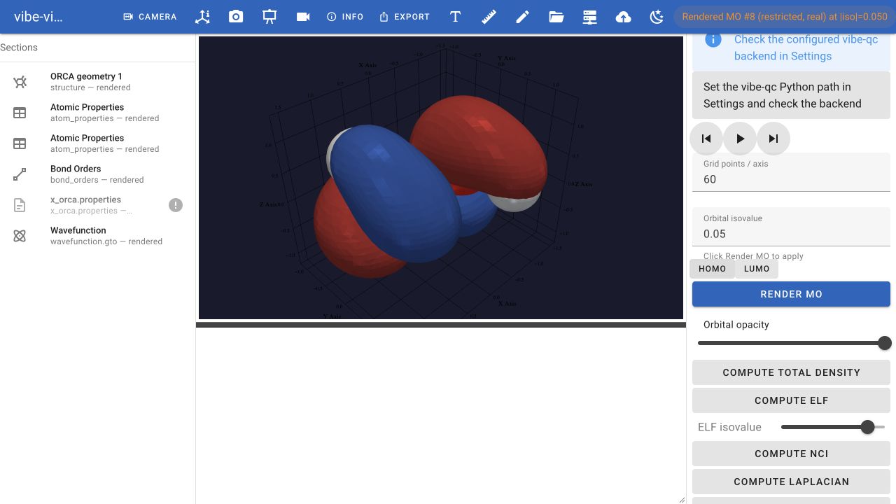
The HOMO belongs to the new displaced-geometry calculation. The optional vibe-qc backend controls are for additional operations such as localization; rendering these archived ORCA orbitals does not require that backend.

7. Select the first Atomic Properties section and check Method → Mulliken. The table lists charges in input atom order: O, O, H, H. The second section contains Löwdin charges; Bond Orders contains the imported Mayer analysis.

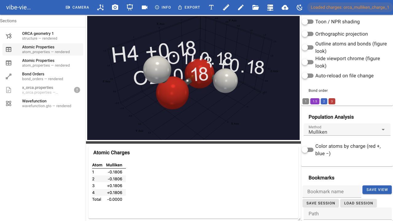
The charge table and atom labels refer to the newly calculated dataset.

Quantity	ORCA output for the displaced single point
Final energy / Eh	−151.264448448530
Energy above the original optimized geometry / Eh	+0.005684679314
Dipole magnitude / D	1.9381
Mulliken charge, O 1 / e	−0.180605
Mulliken charge, O 2 / e	−0.180623
Mulliken charge, H 3 / e	+0.180608
Mulliken charge, H 4 / e	+0.180620

The coordinate, orbital-energy and charge comparisons passed against the submitted input and printed ORCA output. The browser check exercised both frontier-orbital renders, the structure and the Mulliken table. This run used command-line vq submission/fetch followed by browser inspection.

The modes were combined from the archived equilibrium geometry, not added repeatedly to the last edit. Each signed amplitude sets the longest atomic vector of that mode; the final sum is not rescaled. This prepares a chosen distortion, not an IRC path or an optimized minimum.

A single point produces no new frequencies, Raman or VCD spectra. Keep peroxide.qvf separately for the original modes and spectra; do not copy its Hessian into the new result directory. To calculate new spectra, prepare a new frequency job for the intended geometry using the options in section 1.

4. Compare the calculated results

The original run contains four atoms, 38 spatial orbitals and 18 electrons. Its final SCF energy is −151.270133127844 Eh. The imported geometry agrees with the optimized XYZ to better than 1e-8 Å. Archive validation passes for both supplied QVFs.

ORCA mode	Wavenumber / cm⁻¹	Raman activity / Å⁴/amu	VCD / 10⁻⁴⁴ esu² cm²	Mirror VCD / same units
6	328.82511	6.7666	+194.95	-194.96
7	911.38108	9.6784	-9.19	+9.19
8	1263.81557	2.4918	+7.24	-7.24
9	1405.45587	9.6360	-8.39	+8.38
10	3637.41726	35.3440	-54.89	+54.90
11	3637.98379	90.8819	+28.83	-28.84

The Hessian prints Raman activities and depolarization ratios to four decimal places; the main output prints six. Imported activities agree with that output within 0.00005 Å⁴/amu. The VCD output prints strengths to two decimal places, which the importer preserves. Frequencies use the more precise Hessian values, matched to each printed table by mode index.

To repeat the mirror check, download the mirrored optimized input and mirror dataset. The input was generated by vibe-view with Frequencies, Raman and VCD enabled, after reflecting every optimized z coordinate. Submit it in its own directory as calculation.inp, using the same vq command and a new job name. No second geometry optimization is needed for this comparison.

The maximum frequency difference was 0.01591 cm⁻¹, the maximum Raman activity difference 0.0081 Å⁴/amu, and the largest residual after adding opposite VCD strengths 0.01 in the table’s units. These are observed numerical differences for this setup, not universal acceptance tolerances.

Both outputs reached ORCA TERMINATED NORMALLY with exit code 0. The original queue job completed; vq classified the mirror job as time_exceeded under the initial five-minute budget despite complete scientific output. The numerical comparison uses those complete files; it is not a claim that the mirror queue lifecycle passed. The commands above allow ten minutes. Check both queue status and output completeness for your own run.

5. Interpret the example

These are harmonic results for one conformer at a modest basis size. They are an import and display example, not an experimental spectrum prediction. The mirror calculation tests handedness: reflection leaves frequencies and Raman activities unchanged within numerical tolerance, while signed VCD rotatory strengths reverse. Equal populations of mirror conformers cancel VCD; do not interpret this single-conformer plot as a net signal for an unresolved mixture.

Keep the original ORCA files. The QVF contains the imported data, not every response tensor or restart record. Neither isotope recalculation, resonance Raman nor anharmonic spectra are implemented by this Hessian importer.

6. Compare both datasets and export spectra

Open the downloaded original and mirror archives together:

vibe-view open peroxide.qvf mirror.qvf

Select VCD Spectrum, enable Compare across open files, leave Normalize off and use Native unit. Both archives have one VCD section with identical units, so their signed strengths can be compared directly. Switch to Raman Spectrum: the two curves should nearly coincide. These are separate calculation datasets; opening them together does not merge opposite-handed structures or average their strengths.

For a numerical export:

1. Turn Compare across open files off and select the intended dataset in Files. Export CSV exports the active dataset, not every overlaid file.

2. Select Native unit, leave Normalize off, and click Export CSV.

3. In the file, distinguish the # envelope block from the # peaks block. The first is the sampled broadened curve; the second contains the discrete source strengths. Broadening changes the envelope, not the peaks.

4. The CSV column is generically named intensity. For this Raman example it means Å⁴/amu activity; for VCD it means rotatory strength in 10⁻⁴⁴ esu² cm². Keep those units with your exported data when importing it into another tool.

5. Repeat for the other dataset. Compare the peak values with the reference table above; the CSV rounds coordinates and strengths to six significant figures, so the archive remains the more precise source.

You can read the stored arrays without a browser or plotting dependency:

from vibeview import QVFReader

with QVFReader("peroxide.qvf") as reader:
    for section_id in ("orca_raman", "orca_vcd"):
        spectrum = reader.read_spectra(section_id)
        print(section_id)
        for label, wavenumber, strength in zip(
            spectrum.labels, spectrum.frequencies, spectrum.intensities
        ):
            print(label, wavenumber, strength)

The printed labels retain ORCA’s zero-based mode indices. Raman includes zero-frequency translational/rotational rows from the Hessian, while VCD contains only the modes printed in its output table. Match by mode label, not by assuming the two arrays have identical row numbers.

7. Resolve missing or unexpected spectra

Symptom	Check and next step
The form rejects Raman/VCD	Select Frequencies or Single Point + Freq + Opt. These options cannot accompany a single point or optimization-only task.
Only IR appears	Check the submitted input, not a later preview: Raman needs Polar 1; VCD needs doVCD true and analytical frequencies. A change in the form does not modify a job already submitted.
Raman appears but VCD does not	Keep stdout.log with the fetched files, or pair a matching calculation.out with calculation.hess. A browser upload of the Hessian alone cannot include the output.
VCD import rejects the output	Check normal termination and fetch the matching Hessian/output from one run. Multiple VCD tables, unknown units and geometry/frequency mismatches are deliberately rejected.
The queue reports time_exceeded	Inspect the log and completeness of the expected files. If incomplete, resubmit in a fresh directory with a larger time budget. A normally terminated ORCA output and a successful queue lifecycle are distinct checks.
VCD is all zero	An achiral structure or cancellation can have zero VCD. Check the conformer and calculation; missing data and calculated zero strengths are different cases.
Peaks near 3638 cm⁻¹ seem to merge	The example has two nearby modes. Use Sticks only or reduce broadening; do not infer a missing mode from the envelope alone.
The chart is too small	Drag Result details upward. Current spectrum plots resize with the panel, including the negative VCD range and axis labels.

If your installed viewer has neither the Raman/VCD input options nor these spectrum sections, check which version you installed. This chapter follows the source version; public release packages and the deployed handbook may lag main. Use a source revision containing the feature, or wait for its release, rather than changing a scientific input to work around an older viewer.