From input to a shareable result
This tutorial turns a small XYZ file into a validated archive, inspects it without a display, and exports results for a colleague. Every input in the first workflow ships with vibe-view. No producer, queue or calculated showcase file is required.
You need: an activated viewer environment. The core profile covers the
commands below; opening the browser needs [viewer], and creating a PNG
needs a working offscreen graphics backend. See Installation.
1. Copy a real input and import it
Run these commands from a directory where you want to keep the results:
vibe-view examples --copy viewer-workshop
cd viewer-workshop
vibe-view import water.xyz -o imported-water.qvf
vibe-view validate imported-water.qvf
vibe-view info imported-water.qvf
The copied water.xyz contains three atoms. The example bundle also
includes a ready-made water.qvf; this tutorial writes imported-water.qvf
so you can follow the import without replacing the bundled archive. Importing it creates one QVF
with a structure section; validation checks the manifest and stored member
digests. Keep the original XYZ too: conversion preserves its geometry, but
does not invent an energy, basis set, electron density or calculation log.
examples --copy and import refuse to overwrite an existing output unless
you pass --force. For another run, use a fresh directory or deliberately
choose new filenames.
File |
Purpose |
|---|---|
|
The original geometry in ångström |
|
A reusable archive with a manifest and member checksums |
|
The bundled example instructions |
For your own files, replace water.xyz with a supported input. Use
vibe-view formats to check which importer is available. A cube can carry a
sampled field; an XYZ cannot. Independent inputs create separate archives.
ORCA companions with the same calculation basename are grouped into one
dataset; see the ORCA tutorial. Input formats lists
what each route preserves.
To calculate electronic properties from a geometry, follow the worked ORCA water example. It includes the exact input and results from a real vq submission, so you can either repeat the calculation or inspect the supplied QVF and compare its orbitals, energy and charges.
2. Inspect before opening a window
vibe-view show imported-water.qvf --labels --size 80x24
vibe-view info imported-water.qvf --json > water-info.json
vibe-view show imported-water.qvf --plain --size 80x24 > water-frame.txt
The terminal view shows one oxygen and two hydrogens, with labels. It works without a display server or OpenGL. The JSON records the section inventory and available metadata; the text file is a portable view for a log or report. Missing calculation metadata is reported as missing, not as zero energy.
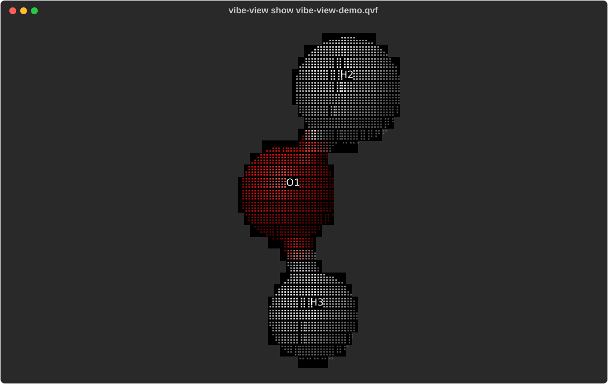
The same bundled water geometry rendered by the real terminal renderer.
The colours require a terminal that supports true colour; --plain omits them.
For interactive inspection, choose one of these commands:
vibe-view open imported-water.qvf
vibe-view tui imported-water.qvf
These are alternatives, not a sequence: each owns its terminal until you stop it. For the browser, use Ctrl+C in the launching terminal; for the TUI, press q. In the browser, drag to rotate and press r to reset. In the TUI, use the arrow keys and r.
3. Export the right result
A numerical archive, a picture and an interactive geometry page serve different purposes. Choose what the recipient needs:
vibe-view export imported-water.qvf -f xyz -o water-export.xyz
vibe-view export imported-water.qvf -f html -o water-view.html
vibe-view export imported-water.qvf -f svg -o water.svg
Output |
Useful for |
What it does not carry |
|---|---|---|
|
Reopening the archived data in the viewer or SDK |
Results the input never contained |
|
Passing the geometry to another program |
QVF metadata, scientific sections and stored connectivity |
|
Rotating the exported structure in a browser without Python |
The full analysis interface; Three.js is loaded from a CDN, so network access is needed |
|
A scalable structure drawing |
Interactive rotation or numerical fields |
To make a PNG, check the graphics backend first:
vibe-view capture-selftest
vibe-view capture imported-water.qvf -o water.png --size 1200x800
The PNG should show all three atoms. If the self-test fails, follow headless setup; converting the input again will not repair a missing graphics backend. For consistent figures across a study, keep size, representation, camera and contour settings fixed and retain the commands used to make each figure.
4. Inspect the same archive from Python
Save the following as inspect_water.py in viewer-workshop/, then run
python inspect_water.py:
from pathlib import Path

from vibeview import QVFReader, get_structure, info, render_terminal, validate

with QVFReader("imported-water.qvf") as reader:
    result = validate(reader)
    if not result["valid"]:
        raise SystemExit(result["error"])
    metadata = info(reader)
    geometry = get_structure(reader)
    print("Atoms:", len(geometry["atoms"]))
    print("Sections:", [(s.id, s.kind) for s in reader.sections])
    print("Energy / Eh:", metadata["scf_energy_eh"])
    Path("water-python.txt").write_text(
        render_terminal(reader, size=(80, 24), plain=True), encoding="utf-8"
    )
Expect three atoms, one structure section, and None for the energy. The
reader is reused for all operations and closed by the context manager.
water-python.txt contains a terminal view. The SDK reference
explains ownership, exceptions and the supported API.
Continue with an ORCA calculation
Keep the calculation’s property file, primary GBW or exported orbital JSON, and MCD files together under their original basenames. In that result directory:
vibe-view import calculation.property.json -o calculation.qvf
vibe-view validate calculation.qvf
vibe-view info calculation.qvf
vibe-view open calculation.qvf
The import gathers matching companions into one archive. A selected GBW needs
the matching orca_2json utility; a property file alone contains no MO
coefficients. Validation checks the archive’s structure and integrity, while
info shows which scientific sections are actually present. The result can
contain a structure, wavefunction, absorption/ECD or raw MCD spectra, charges
and bond orders, depending on the calculation.
The dedicated ORCA chapter walks through preparing these files, selecting orbitals and spectra, inspecting properties, importing Compound steps and sharing results without an ORCA installation.
Continue with a calculated archive
The workshop above ends with geometry. For orbitals, spectra and charges, start with an archive that actually contains them:
vibe-view info calculation.qvf
vibe-view table calculation.qvf
A section’s kind tells you what it means, such as volume.density.
Its ID identifies one section, such as rho_total. Use IDs with
open -s, show -s and capture -s; use a kind with table --kind.
The following examples assume a density whose ID is rho_total and a
charge table of kind atom_properties:
vibe-view open calculation.qvf -s rho_total
vibe-view show calculation.qvf -s rho_total --isovalue 0.05
vibe-view capture calculation.qvf -s rho_total --isovalue 0.05 -o density.png
vibe-view table calculation.qvf --kind atom_properties --format csv > charges.csv
Choose the contour in the field’s recorded units. Orbital sign colours are phase labels; changing the sign of a whole orbital does not change its probability density. A density difference requires compatible underlying fields; comparing two attractive surfaces does not establish that.
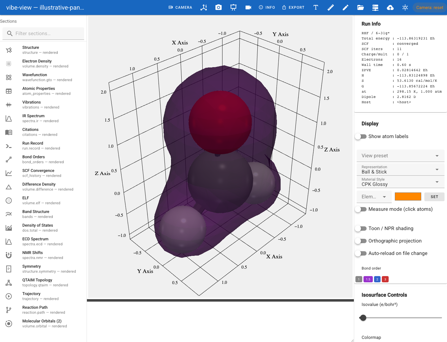
A computed field from a separate formaldehyde showcase calculation. This is an example of the next stage, not a result produced by the water XYZ workflow.
Work remotely
For a quick inspection on a remote machine, install the viewer there and
run show or tui directly. For browser interaction, keep the server on
loopback and forward its port. In a terminal on your laptop:
ssh -L 8090:127.0.0.1:8090 you@remote-host
Then, in that SSH session, activate the remote viewer environment and run:
vibe-view open calculation.qvf --no-browser --port 8090
Open http://127.0.0.1:8090 in your laptop’s browser. Keep the SSH session
open while using the viewer. Stop the viewer with Ctrl+C, then exit the
SSH session when finished. A failed connection is addressed in
browser troubleshooting.
Next workflows
ORCA calculations: open the complete dataset, inspect orbitals and spectra, and share a QVF.
Guided tour: inspect density, orbitals, vibrations and periodic data.
Biomolecules: choose chains, residues and secondary-structure views.
Building and editing: change geometry and export the edited structure.
Figures without a display: batch captures, animation and chart exports.
Python SDK: validate, compare or slice many archives in a script.