Worked example: water through ORCA and vq

For Raman and signed VCD spectra, continue with the hydrogen-peroxide tutorial.

Prepare a water single point in vibe-view, submit it through vq, then open the completed calculation as one dataset. This tutorial uses the geometry and results from a real ORCA 6.1.1 run with PBE/def2-SVP and TightSCF. The submission, result fetching, structure measurements, orbital rendering and Mulliken table were exercised in the browser viewer.

Get the example

Save these files in a new tutorial directory:

• Water geometry — the exact input geometry.

• ORCA input — the input generated by the viewer.

• Calculated QVF — the imported structure, orbitals and properties from the completed run.

To inspect the supplied result: install vibe-view, run vibe-view open water-orca.qvf from your download directory, and start at Inspect the structure. This route needs neither ORCA nor vq. The QVF contains calculated data, not an ORCA executable or a restart file.

To repeat the calculation: use a viewer version with the ORCA calculation form, install vq in the viewer’s Python environment, and register ORCA as the local queue’s orca binary. Follow Prepare vq once. Install the matching orca_2json utility for GBW import; see ORCA setup.

1. Prepare and save the input

Open the downloaded geometry:

vibe-view open water.xyz

Select Structure, open Calculation Parameters, and set:

Control	Value
Calculation engine	ORCA
ORCA method	PBE
ORCA basis	def2-SVP
Calculation Type	Single Point
Charge / Multiplicity	0 / 1
Processes (nprocs)	1
MaxCore (MB per process)	1000

Click Preview ORCA input. The geometry must match this input exactly if you want to compare with the reference values below:

# Generated by vibe-view; Cartesian coordinates in angstrom
! PBE def2-SVP TightSCF SP
%pal nprocs 1 end
%maxcore 1000
* xyz 0 1
O  0.0000000000 0.0000000000 0.0000000000
H  0.0000000000 0.0000000000 0.9572000000
H  0.9266270000 0.0000000000 -0.2399870000
*

Click Save ORCA input (.inp) to keep a copy. If you change the geometry or form, preview again. Submission regenerates the input from the current form; editing a previously downloaded input does not change what this form submits.

2. Submit, fetch and open

1. Click Submit ORCA to vq. In the submission dialog choose a job name such as orca-water and a Wall time (minutes) budget of 5.

2. Check the request: one CPU and 1334 MB queue memory. The memory reservation includes headroom above ORCA’s 1000 MB MaxCore setting.

3. Click Submit to vq. The Job Manager opens. Wait for your job to complete and inspect its log tail for ORCA TERMINATED NORMALLY.

4. Click that job’s Fetch & open results. The viewer fetches the result directory and loads one calculation dataset. A new run has its own queue identifier; select your job rather than an unrelated completed calculation.

In the fetched directory, keep calculation.gbw and calculation.property.txt together. The GBW supplies orbital coefficients; the property file supplies the populations and other properties. vq captures ORCA’s output in stdout.log. Use it for the comparisons below. The viewer combines the companion result files; it does not extract these scientific data from the log.

3. Inspect the structure

Select Structure. You should see one oxygen and two hydrogens. Use Camera → Reset / fit all to frame them, then click the toolbar’s List all bond distances & angles button.

Expect two O–H distances of approximately 0.957 Å and an H–O–H angle of 104.5°. This is a single point, so it preserves the supplied geometry; these are not optimized bond lengths. In the verified import, the largest coordinate difference from the XYZ was below 5e-9 Å.

The sidebar also contains two Atomic Properties entries (Mulliken and Löwdin), Bond Orders, and Wavefunction. The raw x_orca.properties entry is retained metadata without a renderer; its skipped state does not mean the supported properties failed to load.

4. Render the HOMO and LUMO

Select Wavefunction, click HOMO, and click Render MO. Use 60 grid points per axis and orbital isovalue 0.05 to reproduce the example view. If needed, use Camera → Reset / fit all again.

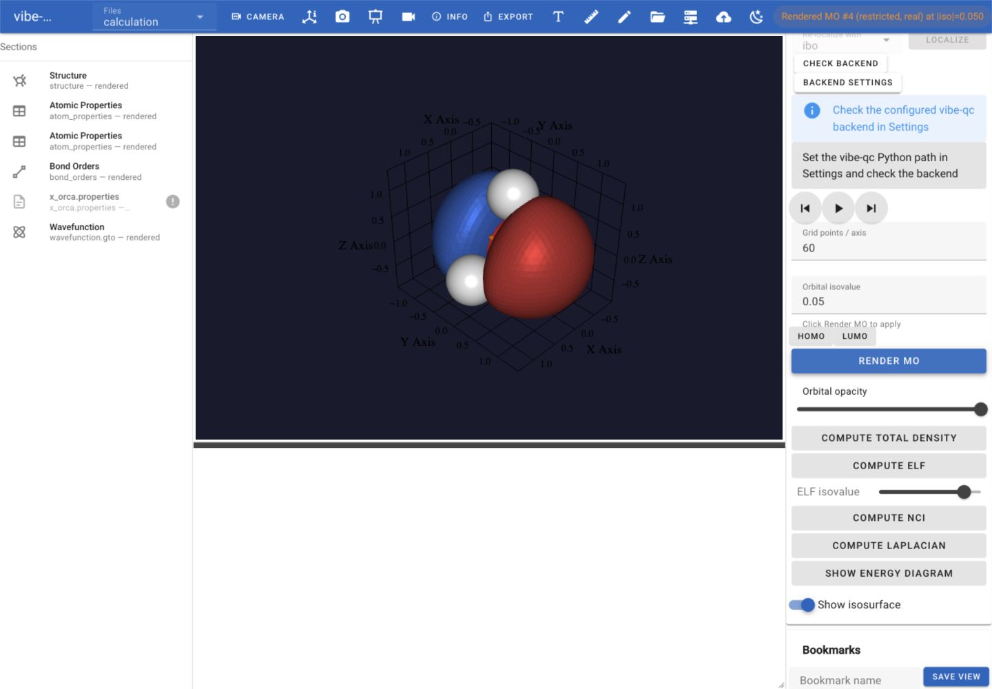
The actual ORCA water HOMO rendered from the fetched GBW. Blue and red denote opposite signs of the orbital, not positive and negative charge.

Repeat with LUMO, then Render MO. The imported wavefunction contains 24 spatial orbitals and ten electrons: the first five orbitals have occupation 2, and the others have occupation 0. The viewer uses zero-based MO indices:

Orbital	Viewer index	Occupation	Reference energy / Eh
HOMO	4	2	−0.2284903806
LUMO	5	0	+0.0300148625

Compare with ORCA’s ORBITAL ENERGIES table in stdout.log, which prints fewer decimal places and, in this run, only the first ten virtual orbitals. The GBW contains all 24. A global reversal of orbital sign does not change the physical orbital.

5. Compare energy, dipole and charges

In Run Info, check SCF convergence, charge/multiplicity 0 / 1, ten electrons and the total energy. Select the Atomic Properties entry whose Method is Mulliken, then read the Atomic Charges table.

Quantity	Reference result
Total energy / Eh	−76.272069187704
O1 Mulliken charge / e	−0.2761619470
H2 Mulliken charge / e	+0.1380807561
H3 Mulliken charge / e	+0.1380811909
Sum of Mulliken charges / e	0, within rounding
Viewer dipole magnitude / D	1.9356375709

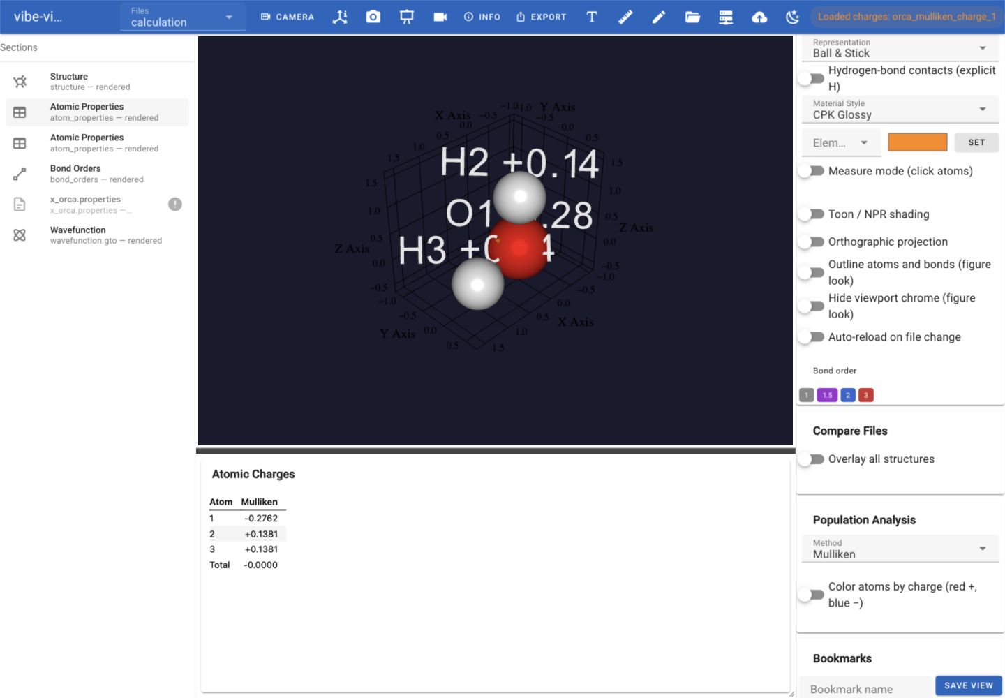
The displayed charge table rounds the imported values to four decimal places.

ORCA prints a dipole magnitude of 1.935676811 D for this run. The approximately 0.00003924 D difference comes from the Debye conversion factor. Comparing in atomic units gives the same vector, approximately (0.602222067, 0, 0.466121587), within 1e-9 a.u.

These numbers describe this geometry, method and ORCA version. A changed geometry, method, numerical setup or version can change the result. For the supplied QVF, the energy agreed with the original log within 1e-10 Eh; printed orbital energies and charges agreed within 5.1e-7 Eh and e, respectively. These are import comparisons, not universal convergence criteria for new calculations.

6. Keep and share your result

From the fetched calculation directory, create your own portable archive:

vibe-view import calculation.property.txt -o my-water-orca.qvf
vibe-view validate my-water-orca.qvf
vibe-view open my-water-orca.qvf

Keep the GBW beside the property file during import. The saved QVF can then be opened on another computer without ORCA. Validation checks archive integrity; the comparisons above check that the imported results agree with the calculation. Keep the original ORCA files for restarting or further analysis.

This single point exercises structure, orbitals and ground-state properties. It does not produce vibrational or electronic spectra. Continue below to run a frequency calculation, or explore ORCA spectra and the broader ORCA chapter.

7. Extend the example to vibrations and IR

Return to the original water.xyz and use the same method, basis, charge, multiplicity and resource settings. Change Calculation Type to Single Point + Freq + Opt; the generated keywords are Opt Freq. Preview the input and submit through vq with a new job name, then Fetch & open results when complete. This optimizes the geometry before calculating its harmonic frequencies, so its energy and charges differ from the single-point example.

The following downloads come from a second real ORCA 6.1.1 PBE/def2-SVP run submitted through vq:

• Optimization/frequency input.

• Native Hessian result for geometry, normal modes and IR without an ORCA installation.

• Complete frequency dataset including the optimization trajectory, final structure, orbitals, properties, vibrations and IR.

To inspect the supplied result immediately:

vibe-view open water-frequencies.qvf

Select Vibrations and choose the mode near 1608 cm⁻¹. Click Play, then Pause; use the phase filmstrip to compare positions at different parts of the oscillation. The default display amplitude exaggerates motion to make it visible. Lower it for a subtler view. Six zero modes are retained ahead of the three molecular vibrations. Compare by frequency or account for the index offset: ORCA mode 6 is Mode 7 in the viewer.

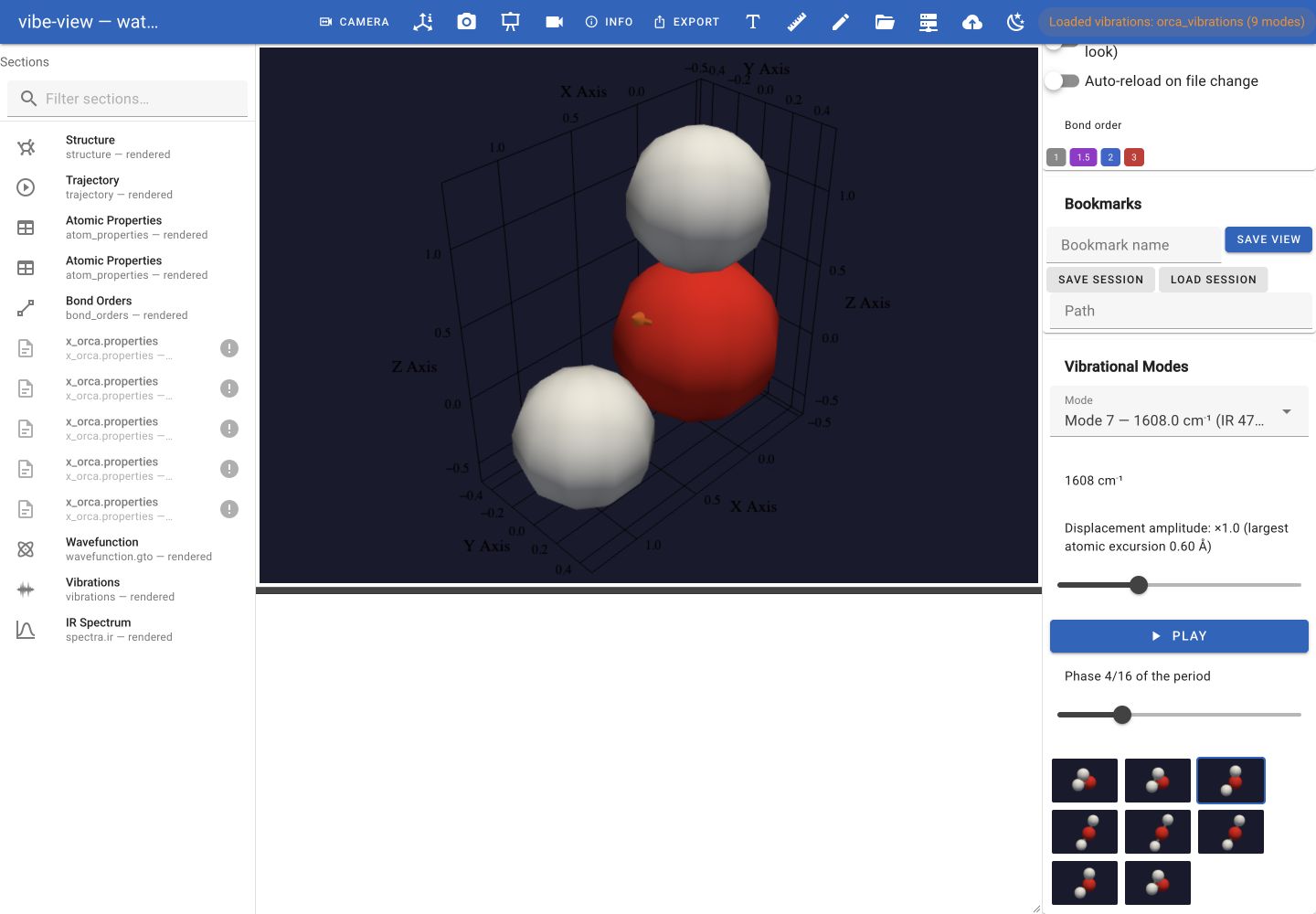
The imported bending mode, paused using the phase filmstrip after playback.

Select IR Spectrum. Keep Normalize off to compare the stick intensities with ORCA’s IR SPECTRUM table. Use Display to show sticks, the broadened envelope or both; Export CSV retains the numerical data. Drag the separator above the result panel upward if the chart needs more room.

ORCA index	Viewer mode	Frequency / cm⁻¹	IR intensity / km mol⁻¹
6	Mode 7	1607.968079	47.49250585
7	Mode 8	3689.749562	2.20520296
8	Mode 9	3788.909314	19.72152928

The frequencies are unscaled harmonic values. The imported intensities agree with ORCA’s printed values at its output precision; they are not the adjacent eps column. The supplied example has no imaginary frequencies. For another system, negative frequencies remain visible and need chemical interpretation before treating the structure as a minimum.

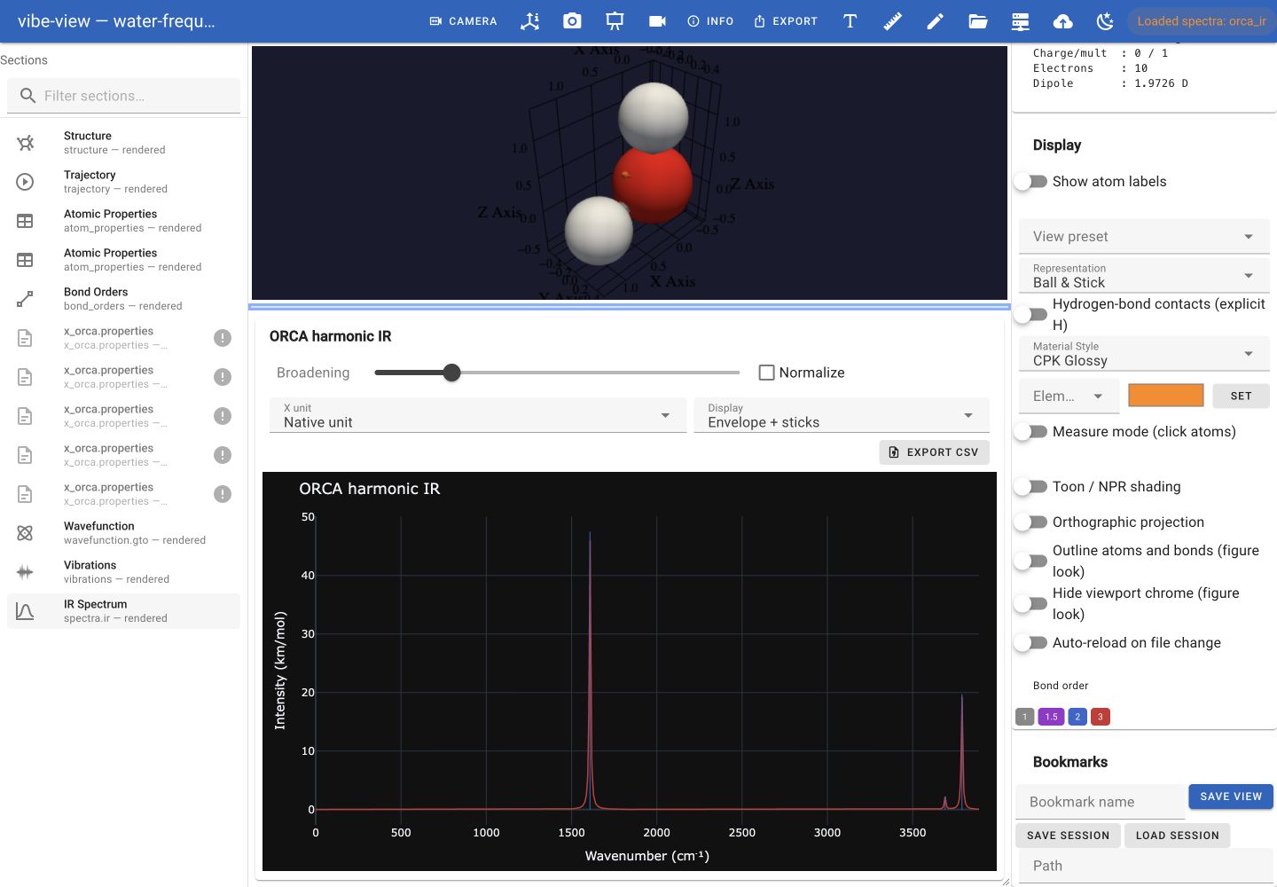
The real frequency calculation’s IR sticks and broadened display in vibe-view.

For your own run, retain calculation.hess beside its property file and GBW when importing to QVF. A .hess opened on its own supplies no orbitals; the complete downloadable QVF above includes them from the matching GBW.