Example outputs
Reference outputs from canonical vibe-qc calculations — the
.out SCF traces, .molden orbital files, and other artefacts
that successful runs produce. Browse to see what success looks
like before you commit to running anything yourself, or download
the bundle to compare against your own runs when something doesn’t
match.
Tip
Every text output starts with the runtime banner — a labelled box
recording vibe-qc version, codename, git revision, and linked
native-library versions. That block is your reproducibility line:
copy it into the SI of any paper that uses vibe-qc to record
exactly which build produced your numbers. Outputs on this page
were regenerated against a clean main commit (banner reads
dev 0.5.0.dev0 "Wilson's Otter"); the v0.5.0 release tag will
re-bundle them with Release v0.5.0 banners.
Tip
Compare your wall-time to the bundled reference. Each run_job
bundle below ships a <basename>.system manifest alongside the
.out file — plain TOML pinning the CPU model, OpenMP thread
count, total RAM, and linked-library versions used to produce that
output. See
Tutorial 29 for the
grep / diff recipes that turn a wall-time number in your
.out into a hardware-aware comparison (“the bundled reference
ran on an M2 Pro at 12 threads in 84 ms — your Xeon at 1 thread
took 1.2 s, that’s the expected ~14× single-thread gap”). The
hostname field is redacted in the bundled outputs; everything
else is full-fidelity. Manifests are documented in
docs/user_guide/output_files.md.
Note
Phase 2 of DOC1 ships the four Level-1 calculations
below. Phases 3-5 add the remaining 10 calculations covering
periodic SCF, NEB, symmetry exploitation, plus VMD-rendered
orbital screenshots and per-tutorial reference outputs. Re-bundle
all of them at any time via
scripts/regenerate_doc_examples.py.
How to read this page
Each calculation gets a card with:
What it does — one-line description of the science.
Files — the bundled artefacts with download links and sizes.
Reproduce — the one-shot command to re-run from the bundled input script.
Highlights — the converged numbers you should expect to see.
The full bundle for each calculation lives under
docs/_static/examples/<slug>/.
Molecular: closed-shell SCF
h2o-rhf — H₂O closed-shell RHF / 6-31G*
The textbook first calculation. Standard molecular Hartree-Fock, single-determinant ground state, ten SCF iterations, ~6 ms wall on a recent machine.
Files (~17 KB total):
input-h2o-rhf.py— input script (496 B)output-h2o-rhf.out— full SCF trace + orbital table + Mulliken / Löwdin charges + Mayer bond orders + dipole + timings (4.4 KB)output-h2o-rhf.molden— MOs for Avogadro / Jmol / Molden (12 KB)
Reproduce locally:
cd ~/path/to/vibeqc/examples
~/path/to/vibeqc/.venv/bin/python input-h2o-rhf.py
Highlights:
Quantity |
Value |
|---|---|
E(SCF) |
−76.003600 Ha |
Converged |
10 iterations |
ε(HOMO) |
−13.46 eV |
ε(LUMO) |
+5.55 eV |
HOMO-LUMO gap |
19.01 eV |
h2o-dft — H₂O RKS / PBE / 6-31G*
Same molecule, same basis, exchange-correlation functional swapped in. Notice the dramatically smaller HOMO-LUMO gap — DFT functionals recover real correlation, the gap shrinks from HF’s overestimate (~19 eV) toward something physically reasonable (~7 eV; experiment is ~6.5 eV for the optical gap).
Files (~18 KB total):
input-h2o-dft.py— inputoutput-h2o-dft.out— full outputoutput-h2o-dft.molden— Kohn-Sham orbitals
Reproduce locally:
cd ~/path/to/vibeqc/examples
~/path/to/vibeqc/.venv/bin/python input-h2o-dft.py
Highlights:
Quantity |
Value |
|---|---|
E(SCF) |
−76.319204 Ha |
ε(HOMO) |
−6.09 eV |
ε(LUMO) |
+0.90 eV |
HOMO-LUMO gap |
6.99 eV |
Molecular: open-shell SCF
oh-radical — Hydroxyl radical UHF / 6-31G*
Open-shell unrestricted Hartree-Fock on a doublet (one unpaired
electron). The setup is the canonical demonstration that spin
information lives on the Molecule (multiplicity=2 here),
not on a separate UHFOptions.spin field — vibe-qc was
deliberately designed without the latter so every RHF / UHF / RKS
/ UKS run on the same Molecule is consistent.
Files (~26 KB total):
input-oh-radical.py— inputoutput-oh-radical.out— full output, alpha/beta orbital tables side by sideoutput-oh-radical.molden— alpha + beta orbitals
Reproduce locally:
cd ~/path/to/vibeqc/examples
~/path/to/vibeqc/.venv/bin/python input-oh-radical.py
Highlights:
Quantity |
Value |
|---|---|
Multiplicity |
2 (doublet) |
α gap (HOMO-α → LUMO-α) |
20.96 eV |
β gap (HOMO-β → LUMO-β) |
17.32 eV |
The alpha/beta gap split is itself the open-shell signature: in a doublet, one of the two HOMOs is singly occupied (the SOMO), so the alpha and beta orbital sets converge to slightly different eigenvalues. RHF would force them equal and miss this physics.
Molecular: geometry optimization
h2o-opt — H₂O relaxation at HF / 6-31G*
Single-water geometry optimization via ASE’s BFGS driver. Starts
from a slightly distorted h2o.xyz and relaxes to the HF/6-31G*
local minimum (fmax=0.01 eV/Å, ~5 BFGS steps). The trajectory
is the classic “watch the bond angle close” animation.
Files (~20 KB total):
input-h2o-opt.py— inputoutput-h2o-opt.out— initial geometry, optimizer steps, final SCF, optimized geometryoutput-h2o-opt.molden— orbitals at the optimized geometryoutput-h2o-opt.traj— ASE trajectory (open withase gui)
Reproduce locally:
cd ~/path/to/vibeqc/examples
~/path/to/vibeqc/.venv/bin/python input-h2o-opt.py
Highlights:
Quantity |
Value |
|---|---|
E (final, RHF/6-31G*) |
−76.009341 Ha |
Final-step SCF |
10 iterations |
|
0.01 eV/Å |
h2o-dimer-opt — Water dimer at HF / 6-31G*
Two waters in a Cs-symmetric H-bonded geometry, BFGS-relaxed at HF/6-31G*. The relaxed R(O…O) is ~2.98 Å — HF overestimates slightly compared to high-level reference (~2.91 Å); for quantitative work add D3(BJ) dispersion or move to MP2.
Files (~53 KB total):
input-h2o-dimer-opt.py— inputoutput-h2o-dimer-opt.out— full optimizer + SCF logoutput-h2o-dimer-opt.molden— orbitals at the minimumoutput-h2o-dimer-opt.traj— relaxation trajectory
Reproduce locally:
cd ~/path/to/vibeqc/examples
~/path/to/vibeqc/.venv/bin/python input-h2o-dimer-opt.py
Highlights:
Quantity |
Value |
|---|---|
E (relaxed, RHF/6-31G*) |
−152.026435 Ha |
Final-step SCF |
12 iterations |
Interaction energy at HF/6-31G* |
~−5 kcal/mol (HF underestimates without dispersion) |
h2o-trimer-opt — Water trimer at HF / 6-31G*
Three waters in a cyclic H-bonded ring, the model system for cooperative H-bonding effects in liquid water. Relaxes to the classic three-fold symmetric structure with ~85° HOH-H angles.
Files (~121 KB total):
input-h2o-trimer-opt.py— inputoutput-h2o-trimer-opt.out— full outputoutput-h2o-trimer-opt.molden— orbitals at the minimumoutput-h2o-trimer-opt.traj— relaxation trajectory
Reproduce locally (~5-10 min wall on a recent laptop):
cd ~/path/to/vibeqc/examples
~/path/to/vibeqc/.venv/bin/python input-h2o-trimer-opt.py
Highlights:
Quantity |
Value |
|---|---|
E (relaxed, RHF/6-31G*) |
−228.051135 Ha |
Final-step SCF |
12 iterations |
Cooperativity ΔE vs 3 dimers |
(a positive ~1-2 kcal/mol three-body term in real life; HF/6-31G* gets the sign but not the magnitude) |
Molecular: numerical-stability stress tests
h2-tight-canonical-orth — Near-linearly-dependent AO basis
H₂ at R = 0.5 bohr (artificially short — the equilibrium is 1.4 bohr) with the diffuse aug-cc-pVTZ basis. The two atoms’ diffuse primitives overlap so heavily that the overlap matrix S is on the edge of singularity (min eigenvalue ~1.86 × 10⁻⁷, condition number ~2.78 × 10⁷). Pre-canonical-orthogonalisation, the RHF driver aborted with “AO basis is linearly dependent” on this kind of input; the new path projects out the linearly-dependent combinations and converges cleanly.
Files (~6 KB total):
input-h2-tight-canonical-orth.py— inputstdout.txt— captured stdout — diagnostic + threshold sweep table
Reproduce locally:
cd ~/path/to/vibeqc/examples
~/path/to/vibeqc/.venv/bin/python input-h2-tight-canonical-orth.py
Highlights:
Quantity |
Value |
|---|---|
Basis dimension |
46 functions |
min eigenvalue of S |
1.86 × 10⁻⁷ |
Condition number |
2.78 × 10⁷ |
Eigenvalues below 10⁻⁶ warn threshold |
1 |
The threshold sweep (1e-9 → 1e-3) shows the kept-MO count drop as canonical orthogonalisation projects out more near-null combinations — total energy stays stable to ~µHa across the whole range, which is the contract: the projection should be numerically inert on a converged calculation.
Visualization
h2o-cube — H₂O HOMO/LUMO/density cube generation
Writes the H₂O HOMO, LUMO, and total electron density to Gaussian
.cube files at fine resolution (spacing=0.15 bohr, 5-bohr
padding) suitable for publication-quality renderings in VMD /
Avogadro / PyMOL / ChimeraX.
Warning
The actual cube files are not bundled here — they’re 6-24 MB each at the documented grid spacing, far over the docs static-asset budget, and useless on a static docs site (you can’t render a cube file in your browser). What ships below is the input script + the captured stdout listing grid sizes and per-cube write timings; a VMD-rendered PNG screenshot will be added in Phase 4 of DOC1.
Files (~2 KB total):
input-h2o-cube.py— inputstdout.txt— captured stdout (grid + write-time info)
Reproduce locally (produces 4 cubes, ~42 MB total):
cd ~/path/to/vibeqc/examples
~/path/to/vibeqc/.venv/bin/python input-h2o-cube.py
Highlights:
The script writes four cube files:
File |
Volume |
Size at default grid |
|---|---|---|
|
total ρ(r) |
~6 MB |
|
HOMO |
~6 MB |
|
LUMO |
~6 MB |
|
multi-volume HOMO−1 → LUMO+1 (4 orbitals) |
~24 MB |
Open in VMD with vmd output-h2o-mo-homo.cube and add an
“Isosurface” representation at isovalue ±0.05 to see the H₂O π
lone-pair lobes.
Periodic: 1D systems
h-chain-uniform — 1D H₂ molecular crystal at uniform spacing
A 1D periodic H₂ chain in a 6-bohr unit cell, with 30 bohr of vacuum perpendicular to the chain to suppress inter-wire interactions. Multi-k convergence: total energy as a function of the k-mesh size, the standard “is my k-mesh fine enough?” demonstration. Each H₂ is a closed-shell bonded pair, so this is a trivial band insulator that converges in a handful of SCF iterations.
Files (~16 KB total):
input-h-chain-uniform.py— inputoutput-h-chain-uniform.out— banner + per-k-mesh SCF traces + convergence table
Reproduce locally:
cd ~/path/to/vibeqc/examples
~/path/to/vibeqc/.venv/bin/python input-h-chain-uniform.py
Highlights:
k-mesh |
E per cell |
Comment |
|---|---|---|
Γ-only (1×1×1) |
−1.265 Ha |
unconverged |
9×1×1 |
−1.131 Ha |
converged to ~µHa |
17×1×1 |
−1.131 Ha |
bit-identical to 9×1×1 → meshconverged |
Demonstrates the universal periodic-SCF rule: sweep the k-mesh until the total energy stops moving, then trust that mesh for production work.
h-chain-peierls — 1D H-chain Peierls-distortion scan
The famous Peierls instability — at the half-filled level, a metallic 1D chain spontaneously dimerises into a band insulator, opening a gap and lowering the total energy. This script scans the dimerisation parameter δ (from uniform δ=0 to maximal δ=1.10 bohr, where alternate H-H distances are 1.4 and 3.6 bohr) and reports the per-cell energy. The driver demonstrates that uniform spacing fails to converge (metal at the Γ point + DIIS oscillation) — only the gapped, dimerised structures converge in sub-100 iterations.
Files (~31 KB total):
input-h-chain-peierls.py— inputoutput-h-chain-peierls.out— full SCF traces + dimerisation-scan table
Reproduce locally:
cd ~/path/to/vibeqc/examples
~/path/to/vibeqc/.venv/bin/python input-h-chain-peierls.py
Highlights:
δ (bohr) |
R short / R long |
E per cell |
Converged? |
|---|---|---|---|
0.00 |
2.500 / 2.500 |
−1.034 Ha |
NO (metal — Peierls-unstable) |
0.40 |
2.100 / 2.900 |
−1.071 Ha |
NO |
0.80 |
1.700 / 3.300 |
−1.112 Ha |
yes (39 iters) |
1.10 |
1.400 / 3.600 |
−1.128 Ha |
yes (27 iters) |
The lowest energy is the most-dimerised structure at δ = 1.10, which is the (somewhat exaggerated) molecular-H₂-crystal limit. The Peierls instability is real and SCF actively can’t converge on the metallic uniform case — this is the textbook “use Fermi smearing or accept the band insulator” lesson.
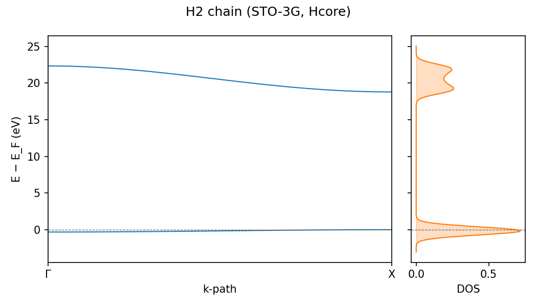
h-chain-bands — Hydrogen-chain band structure
Computes the full band structure E(k) along Γ → X for a uniform H-chain, plus the density of states (k-mesh integration). The output PNG is the band-structure figure used in the docs site’s periodic-SCF tutorial.
Files (~34 KB total):
input-h-chain-bands.py— inputoutput-h-chain-bands.png— band structure + DOS figurestdout.txt— captured stdout (band gap, DOS extrema)
Reproduce locally:
cd ~/path/to/vibeqc/examples
~/path/to/vibeqc/.venv/bin/python input-h-chain-bands.py
Highlights:
The figure shows two bands crossing at Γ — the half-filled metallic regime that Peierls-distorts. The DOS spike at E = ε(Γ) is the 1D van Hove singularity (DOS ~ |E - ε|⁻¹ in 1D).
Periodic: 3D crystals
madelung-constants — Ewald-summed Madelung constants
Vibe-qc’s production Ewald summer (user guide) applied to four canonical ionic crystals. The Madelung constant captures the electrostatic cohesion of an ionic point-charge lattice — a foundational solid-state number, conditionally convergent in real space, absolutely convergent under Ewald splitting. Eight-digit agreement with textbook values.
Files (~6 KB total):
input-madelung-constants.py— inputoutput-madelung-constants.out— table of computed vs reference Madelung constants
Reproduce locally:
cd ~/path/to/vibeqc/examples
~/path/to/vibeqc/.venv/bin/python input-madelung-constants.py
Highlights:
Crystal |
Computed M |
Reference |
Δ |
|---|---|---|---|
NaCl (rocksalt) |
1.7475645946 |
1.7475645946 (Crandall 1987) |
6 × 10⁻¹² |
CsCl |
1.7626747729 |
1.7626747 (Tosi 1964) |
3 × 10⁻⁹ |
ZnS (zincblende) |
1.6380550534 |
1.6380 (Sakamoto 1955) |
5 × 10⁻⁵ |
The accuracy on NaCl + CsCl (8-12 digits) is set by the Ewald
omega and cutoff parameters. The looser ZnS agreement is the
limit of the published reference value — vibe-qc agrees with
itself to 10 digits across multiple ω.
nacl-symmetry — NaCl Pm-3m symmetry exploitation
Builds the LatticeMatrixSet (overlap matrix) for NaCl with a 20-bohr cutoff, attaches the full Pm-3m space group (48 operations) via spglib, and compresses-and-reconstructs via the atom-pair-orbit symmetry path. Reports compression ratio and machine-precision round-trip error — the foundation for the upcoming SYM2c symmetry-aware periodic SCF (v0.6+ wall-clock optimization).
Files (~7 KB total):
input-nacl-symmetry.py— inputstdout.txt— captured stdout
Reproduce locally:
cd ~/path/to/vibeqc/examples
~/path/to/vibeqc/.venv/bin/python input-nacl-symmetry.py
Highlights:
Quantity |
Value |
|---|---|
Space group |
Pm-3m, 48 operations |
n cells × n atom-pairs |
2060 (515 cells × 4) |
n symmetry orbits |
108 |
Compression ratio |
19.07× |
Max block error (round-trip) |
4.4 × 10⁻¹⁶ (machine precision) |
The compression ratio shows that out of 2060 atom-pair triples, only 108 are independent under Pm-3m — the rest are related by symmetry. SYM2c will turn this into a 19× wall-clock speedup on high-symmetry SCF builds.
Method showcases
nh3-umbrella-neb — NH₃ umbrella inversion via NEB
Climbing-image Nudged Elastic Band located at the planar D₃h transition state for ammonia umbrella inversion. Chains together endpoint optimization (BFGSLineSearch on both enantiomers), NEB band setup with 5 intermediate images, and FIRE optimization to the transition state.
Files (~9 KB total):
input-nh3-umbrella-neb.py— inputoutput-nh3-umbrella-neb.out— endpoint optimisations + NEB log + MEP energies + TS geometryoutput-nh3-umbrella-neb.traj— full reaction path (open withase gui)
Reproduce locally (~3-5 min wall):
cd ~/path/to/vibeqc/examples
~/path/to/vibeqc/.venv/bin/python input-nh3-umbrella-neb.py
Highlights:
Quantity |
Value |
|---|---|
Method |
HF / STO-3G |
Computed barrier |
0.483 eV (11.14 kcal/mol) |
Experimental |
~5.8 kcal/mol |
Discrepancy |
HF/STO-3G’s classic ~2× over-estimate of inversion barriers |
This is a qualitative demonstration — HF + minimal basis
overshoots the barrier by ~2×, the well-known limitation of the
combination on inversion problems. For quantitative thermochemistry
move to MP2 or hybrid DFT in a def2-TZVP basis (run_job(method= "rks", functional="B3LYP", basis="def2-tzvp") on the same NEB
setup).
ASE workflows (Phase D)
Pure-ASE workflows where vibe-qc is the backing calculator —
runnable with pip install '.[ase]' and no other QC code. Each
script demonstrates an ASE-native idiom (BFGS, Vibrations, NEB,
Velocity-Verlet) plugging straight into our calculator without
glue.
ase-bfgs-h2o-opt — geometry optimization via ASE BFGS
ASE’s BFGS driver pulls forces from vibeqc.ase.VibeQC,
relaxes H₂O to its HF/6-31G* minimum in ~6 steps. Plots
energy + |F|max convergence per step.
Output: convergence PNG + per-step trajectory + log
ase-vibrations-h2o — vibrational analysis via ASE Vibrations
ase.vibrations.Vibrations does FD on top of vibe-qc’s analytic
forces. The three real frequencies on H₂O / 6-31G* fall in the
expected HF-overshoot band (bend ≳ 1500 cm⁻¹, two stretches
3500-4500 cm⁻¹).
Script:
examples/ase_workflows/vibrations-via-ase-vibrations.pyOutput: per-displacement SCF cache (resumable) + frequencies summary
ase-neb-nh3 — NEB transition-state via vibe-qc only
NH₃ umbrella inversion through vibe-qc’s calculator end-to-end. Climbing-image NEB on 5 intermediates, FIRE optimizer, MEP plot with TS marked.
Output: MEP CSV + plot
ase-md-water-nve — NVE MD energy-conservation diagnostic
Velocity-Verlet on H₂O / RHF / STO-3G, 50 steps × 0.5 fs. Headline result: |ΔE_tot| < 10 meV over 25 fs — vibe-qc’s analytic forces are numerically consistent with its energy gradient. The textbook MD-driver-validation test.
Output: time-series CSV + energy-conservation plot + .traj
ase-surface-h2-pt111 — placeholder for v0.5+
Pt(111) 4-layer slab + atop H₂ via ase.build.fcc111. Sets up
the geometry, points at the intended VibeQCPeriodic
calculator + BFGS workflow, exits cleanly with a “needs G1/G2”
notice.
Script:
examples/ase_workflows/surface-h2-pt111-singlepoint.pyOutput: bare geometry (XYZ) — placeholder until G1/G2 ship in v0.5
Cross-validation against external codes (Phase E)
Same chemistry, multiple QC codes, comparison table. The
:mod:vibeqc.benchmark framework wraps vibe-qc, PySCF, and
(optionally) ORCA / Psi4 / Gaussian / NWChem into a single
compare_calculators(...) call. Scripts run cleanly in degraded
mode (fewer codes installed → fewer rows) and full mode (all
codes available → full table). All assert agreement to a
documented tolerance.
Tip
Verified result on the v0.5 development machine: vibe-qc / PySCF / ORCA agree on H₂O / RHF across STO-3G → 6-31G* → cc-pVDZ → cc-pVTZ → def2-TZVP to 0.0001 meV (~0.04 µHa). That’s chemistry-grade cross-validation in <30 seconds wall.
compare-h2o-hf — H₂O / RHF / 6-31G* across vibe-qc + PySCF + ORCA
The minimal cross-validation. Tight tolerance (1e-5 eV / 1e-4 eV·Å⁻¹) since the SCF skeleton is identical.
Side-by-side bundle (~96 KB) — download both sides and compare input/output line-for-line:
compare-h2o-hf.py— the cross-validation driverstdout.txt— captured comparison tableoutput-compare-h2o-hf.csv— CSV with per-row energies + forcesvibe-qc side (
vibeqc/):ORCA side (
orca/):orca.inp— the 5-line ORCA input ASE generatedorca.out— full ORCA logorca.engrad— gradient file
compare-h2o-dft — H₂O / RKS-PBE / 6-31G* DFT cross-check
Same DFT functional through three independent grid implementations. Loose tolerance (5 mHa) — per-code DFT-grid choices contribute the residual. Adds dipole comparison.
Side-by-side bundle (~100 KB):
compare-h2o-dft.py— driverstdout.txt— comparison tablevibe-qc side:
input-h2o-dft.py,output-h2o-dft.out,output-h2o-dft.moldenORCA side:
orca.inp,orca.out,orca.engrad
Source: examples/ase_compare/compare-h2o-dft.py.
Tip
The vibeqc/ and orca/ subdirs are designed for diff-ing
side by side. Open the two .out files in tabs (or in diff -y if you’re a terminal person) to see how each code formats
the SCF iteration log, banner, and final energy. The two .inp
files (vibe-qc Python script vs ORCA !-line input) are a
useful “convention rosetta” — same chemistry, two input
languages.
The bundle ships only the text artefacts from the ORCA side
(.inp, .out, .engrad). The binary wavefunction
(.gbw, hundreds of KB to MB per system) is excluded — re-run
orca orca.inp from the bundle to regenerate it locally.
Vibe-qc’s own .hess export ships now via
vq.write_orca_hess (Phase M1) — see the
compare-h2o-vibrations bundle below for a side-by-side
.hess comparison.
compare-h2o-vibrations — H₂O analytic Hessian + frequencies vs ORCA
Vibe-qc’s analytic CPHF Hessian (RHF closed-shell) compared
directly with ORCA’s ! HF 6-31G* Freq. Same CPHF formalism, same
basis, same SCF threshold → ~0.5 cm⁻¹ worst-case agreement on
the three real vibrational frequencies (out of ~3800 cm⁻¹ total —
that’s 0.012%).
Side-by-side bundle (~91 KB):
compare-h2o-vibrations.py— driverstdout.txt— table with both frequency vectorsvibe-qc side (
vibeqc/):input-h2o-vibrations.py— RHF + analytic Hessian +vq.write_orca_hessoutput-h2o-vibrations.molden— orbitals + [FREQ] / [FR-COORD] blocksoutput-h2o-vibrations.hess— ORCA-format ASCII (engineering’s M1 export); identical format to ORCA’s, so moltui / chemcraft / VMD-nmwiz read either side
ORCA side (
orca/):
Headline result (verified end-to-end on this machine):
Mode |
vibe-qc (cm⁻¹) |
ORCA (cm⁻¹) |
|Δ| |
|---|---|---|---|
bend |
1884.413 |
1884.869 |
0.457 |
asym stretch |
3777.281 |
3777.635 |
0.354 |
sym stretch |
3877.624 |
3877.774 |
0.150 |
Source: examples/ase_compare/compare-h2o-vibrations.py.
Tip
Side-by-side .hess viewing: drop both .hess files into
moltui to see the same modes from each code’s eigenvectors:
moltui compare-h2o-vibrations/vibeqc/output-h2o-vibrations.hess
# then re-run from the same bundle's orca/ directory:
cd compare-h2o-vibrations/orca && orca orca.inp
moltui compare-h2o-vibrations/orca/orca.hess
ORCA’s .hess isn’t shipped in the bundle (per the
no-redistribute-ORCA-binaries-or-derived-binaries policy
embedded in regenerate_compare_bundles.py); re-run ORCA from
the bundled .inp to regenerate it locally. Vibe-qc’s .hess
ships freely (MPL-2.0 — “outputs are yours”).
compare-water-dimer-dispersion — D3(BJ) consistency on water dimer
Both vibe-qc and ORCA implement D3-BJ from the same Grimme parameter set. The dispersion contribution (interaction energy with D3 minus without) should match to <0.01 kcal/mol — same parameters, same damping function, same atom-pair sum. This script asserts that.
Script:
examples/ase_compare/compare-water-dimer-dispersion.pyOutput: per-monomer + per-dimer + interaction-energy table, with-and-without-D3 panels
compare-basis-convergence — 5 basis sets × 3 codes
H₂O / RHF across STO-3G → 6-31G* → cc-pVDZ → cc-pVTZ → def2-TZVP. Wide table, asserts <1 meV cross-code agreement at every basis. Headline: 0.0001 meV worst case.
Output: convergence CSV + plot
Bundled plot:
output-compare-basis-convergence.png
compare-nh3-neb-barrier — NEB barrier vs ORCA
Full NH₃ inversion NEB through vibe-qc and ORCA, comparing barrier heights. Asserts agreement to 1 kcal/mol on the same NEB-CI protocol.
Output: per-image MEP comparison + plot
Coming in later phases of DOC1
Phase 2 + Phase 3 (this snapshot) ship all 14 text-output bundles above. Remaining phases:
Phase 4 — VMD-rendered PNG screenshots for the cube visualization calculations:
h2o-cubedensity + HOMO + LUMO viavmd -dispdev text -e render.tcl. Each subdirectory will carry its ownrender.tclso screenshots are reproducible from the bundled cube file. Periodic Bloch-density screenshots (lih-chain-bloch-density.pyfromexamples/plots/) come at the same time.Phase 5 — per-tutorial “Reference output” appendix: each of the 25 numbered tutorials gets a 30-line excerpt from the matching bundled output (banner + final energy + key timings) inline at the bottom of the page, with a download link to the full file.
Phase 6 — release-process integration is already in place (release_process.md “Cutting a release” checklist, step 3); final size verification + freeze comes when v0.5.0 tags.
Once Phase 5 lands, every calculation in the documentation has a known-good reference output you can diff against your own run when something doesn’t match.