Basis-set convergence
Total energies and most properties improve as you move from small basis sets (minimal, split-valence) toward large ones (triple-zeta with diffuse and polarization). This tutorial shows how to run a family of calculations, tabulate the trend, and decide when you’ve hit the point of diminishing returns.
A Dunning-family sweep on water
The correlation-consistent series cc-pVXZ (X = D, T, Q) and its
augmented variants systematically approach the HF and correlation
complete-basis-set (CBS) limit. Run HF on water at each:
from vibeqc import Atom, BasisSet, Molecule, run_rhf

mol = Molecule([
    Atom(8, [ 0.0,  0.00,  0.00]),
    Atom(1, [ 0.0,  1.43, -0.98]),
    Atom(1, [ 0.0, -1.43, -0.98]),
])

print(f"{'basis':12s}  {'nbasis':>6s}  {'E (Ha)':>16s}  {'ΔE (mHa)':>10s}  {'iters':>5s}")
print("-" * 60)

previous = None
for name in ("sto-3g", "cc-pvdz", "cc-pvtz", "cc-pvqz"):
    basis = BasisSet(mol, name)
    r = run_rhf(mol, basis)
    delta = ""
    if previous is not None:
        delta = f"{(r.energy - previous) * 1000:+10.3f}"
    print(f"{name:12s}  {basis.nbasis:6d}  {r.energy:16.8f}  {delta:>10s}  "
          f"{r.n_iter:5d}")
    previous = r.energy
Output:
basis         nbasis           E (Ha)   ΔE (mHa)  iters
------------------------------------------------------------
sto-3g             7       -74.94956615                  8
cc-pvdz           24       -76.02431388   -1074.748     10
cc-pvtz           58       -76.05605100     -31.737     12
cc-pvqz          115       -76.06394333      -7.892     15
Reading across:
ΔEshrinks by roughly 1/3 with each level up — classic asymptotic behavior of the correlation-consistent series. Extrapo- lating to CBS by fitting an exponential in the cardinal number X gives around-76.0676 Haat HF limit.cc-pVTZcaptures 99.96% of the cc-pVQZ improvement for 1/2 the basis functions — a reasonable default for production HF.Timing scales as
O(N^4)in the basis-function count for HF, so doubling the basis multiplies the cost by ~16.
A polarized Pople sweep
A quick “what does polarization do?” experiment:
for name in ("6-31g", "6-31g*", "6-31g**", "6-311g**"):
    basis = BasisSet(mol, name)
    r = run_rhf(mol, basis)
    print(f"{name:14s}  nbasis={basis.nbasis:3d}  E = {r.energy:.6f}")
6-31g         nbasis= 13  E = -75.982973
6-31g*        nbasis= 18  E = -76.006678
6-31g**       nbasis= 24  E = -76.021164
6-311g**      nbasis= 30  E = -76.045115
Adding polarization on heavy atoms (
*) gains ~24 mHa.Adding polarization on hydrogens as well (
**) another ~14 mHa.Going from 6-31 → 6-311 split-valence ~24 mHa.
Diffuse-augmented bases (6-311++g**, aug-cc-pvtz) are
essential for anions, weak-interaction energies, and excited-state
calculations. vibe-qc’s basis library ships them, but their small
exponents can trigger linear-dependency issues in certain tight
geometries; tighten conv_tol_grad and bump max_iter when you
need them.
Properties that converge differently
Total energies are the slowest-converging quantity. Relative energies (reaction energies, barriers) and properties (dipoles, bond orders, frequencies) converge faster because error cancellation helps — but not always monotonically.
from vibeqc import mulliken_charges, dipole_moment

for name in ("cc-pvdz", "cc-pvtz", "cc-pvqz"):
    basis = BasisSet(mol, name)
    r = run_rhf(mol, basis)
    q = mulliken_charges(r, basis, mol)
    mu = dipole_moment(r, basis, mol)
    print(f"{name:14s}  E = {r.energy:.5f}   "
          f"q_O(Mull)= {q[0]:+.3f}   μ(D)= {mu.total_debye:.4f}")
Output:
cc-pvdz         E = -76.02431   q_O(Mull)= -0.269   μ(D)= 1.9131
cc-pvtz         E = -76.05605   q_O(Mull)= -0.471   μ(D)= 1.8847
cc-pvqz         E = -76.06394   q_O(Mull)= -0.497   μ(D)= 1.8648
Observe:
Dipole converges cleanly — within 0.03 D by cc-pVTZ, within 0.02 D at cc-pVQZ. The experimental gas-phase value is 1.855 D; cc-pVQZ HF is already on top of it, but this is partially a cancellation of errors (HF over-polarises, no correlation pulls it back) rather than true convergence.
Mulliken charges are a mess — they wander even within a consistent family. Don’t chase a particular value; use them only for within-set comparisons.
Tabulating the trend in a figure
import numpy as np
import matplotlib.pyplot as plt

basis_names = ["sto-3g", "cc-pvdz", "cc-pvtz", "cc-pvqz"]
nbasis, energies = [], []
for name in basis_names:
    basis = BasisSet(mol, name)
    r = run_rhf(mol, basis)
    nbasis.append(basis.nbasis)
    energies.append(r.energy)

fig, ax = plt.subplots()
ax.plot(nbasis, energies, "o-")
ax.set_xlabel("Number of basis functions")
ax.set_ylabel("E(RHF) / Ha")
ax.set_xscale("log")
for n, e, name in zip(nbasis, energies, basis_names):
    ax.annotate(name, (n, e), xytext=(4, 4), textcoords="offset points")
fig.tight_layout()
fig.savefig("h2o_basis_convergence.png", dpi=150)
For a three-point cc-pVXZ extrapolation to the HF CBS limit, fit
E(X) = E_CBS + A * exp(-α X) with α ≈ 1.63 (Halkier et al.
1998).
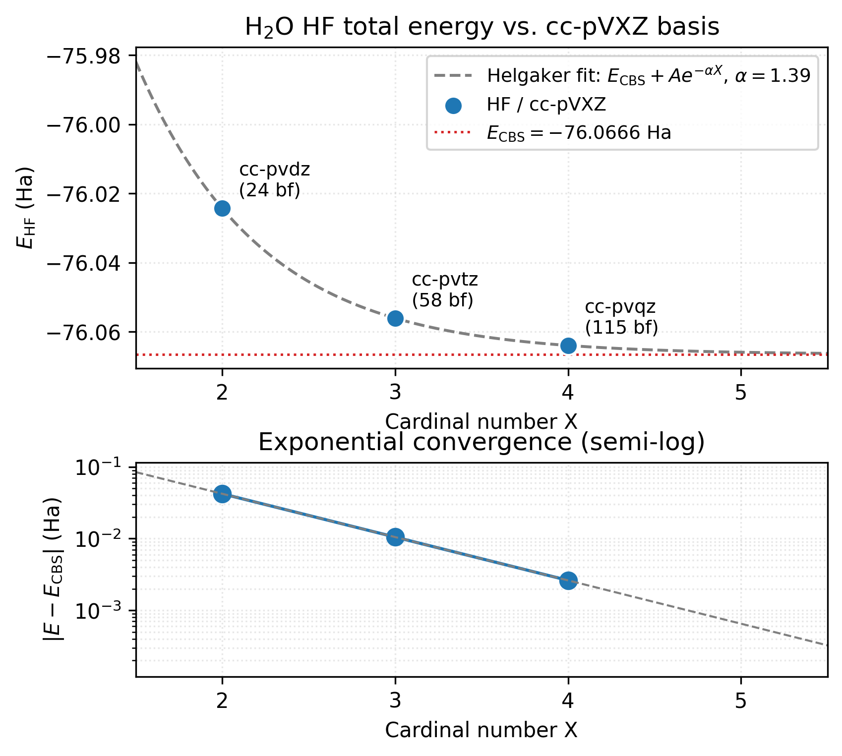
The top panel shows the three cc-pVXZ data points (blue dots) and the fitted Helgaker exponential (grey dashed). The fit’s CBS asymptote sits at \(E_\mathrm{CBS} = -76.067\) Ha (red dotted line) — about 2.6 mHa below cc-pVQZ’s \(-76.064\) Ha. Each level recovers roughly \(1/3\) of what its predecessor missed, so cc-pVQZ has already captured ~99 % of the gap to CBS. The bottom panel makes the rate of convergence explicit: \(|E - E_\mathrm{CBS}|\) falls along an essentially straight line on a semi-log axis, the signature of true exponential convergence. That straightness is the formal justification for trusting the three-point extrapolation: the geometric ratio is constant, so a fit on three consecutive points can read out the asymptote reliably. A correlation-energy plot would look very different — the inverse-cubic \(X^{-3}\) falloff curves gently on semi-log instead of going straight, requiring a different fit form. (See the references for the inverse-cubic correlation extrapolation.)
The figure is regenerated by
examples/plots/water-basis-convergence.py.
Notes
Basis-set superposition error (BSSE) matters for interaction-energy calculations on weakly-bound complexes. No counterpoise correction is built in yet, but you can compute it manually by running the monomer calculations in the dimer basis and subtracting.
Basis linear dependencies. At very large bases (
aug-cc-pVQZand bigger, or diffuse functions in close-packed geometries) the overlap matrix becomes nearly singular. vibe-qc will still converge, but the MO coefficients become noisy. For periodic calculations this is why thepob-*solid-state basis family exists — small-exponent primitives trimmed deliberately.
Theory
What a basis set is
In a practical electronic-structure calculation, every molecular orbital is expanded in a fixed, finite set of atom-centered basis functions \(\{\chi_\mu\}\):
With an infinite, complete basis you get the exact answer of whatever method you’re using (HF, DFT, CCSD, …). With a finite basis you get an approximation whose error scales with basis size; the study of that scaling is basis-set convergence.
Each \(\chi_\mu\) in vibe-qc is a contracted Gaussian-type orbital:
a fixed linear combination of \(K_\mu\) primitive Gaussians with pre-determined exponents \(\alpha_{\mu p}\) and contraction coefficients \(d_{\mu p}\), multiplied by a solid harmonic \((\mathbf{r} - \mathbf{R}_A)^{\ell_\mu}\). The contraction saves the SCF driver from having to optimize every primitive separately — the basis-set designer has already done that for atomic ground states and frozen the inner-shell mix.
Two common hierarchies
Pople split-valence (6-31G*, 6-311G**). Inner-shell contracted
to one function, valence split into two (6-31G) or three (6-311G).
Polarization functions (the * = d-type on heavy atoms; ** = d
p on hydrogen) give radial flexibility beyond the valence’s \(\ell\)-range. Diffuse functions (
+on heavy atoms;++with H) add small-exponent primitives for anions / Rydberg states / weak bonds.
Correlation-consistent (cc-pVXZ). Designed by Dunning to systematically recover correlation energy, with the X = D, T, Q, 5, 6 cardinal number controlling both valence-flexibility and polarization depth together. The key property: the incremental basis-set-error contribution falls off geometrically with X, so two successive cardinal numbers extrapolate reliably to the complete-basis-set (CBS) limit.
Helgaker’s CBS extrapolation
The canonical extrapolation of the HF total energy uses the exponential Helgaker-Klopper-Koch form:
with \(\alpha \approx 1.63\) fixed across the Dunning cc-pVXZ series. Correlation energies converge more slowly (electron-electron cusps), and the standard fit is the inverse-cubic power law
Three consecutive cc-pVXZ points are enough to fit either form.
Polarization functions: what they add
A minimal basis (STO-3G) has no angular-momentum flexibility beyond
what atomic ground states need. Adding a \(d\)-type shell to a heavy
atom, or a \(p\)-type to hydrogen, lets the orbital “polarize” in
response to the bonding environment. Without polarization, oxygen
can’t respond to the electronic asymmetry of the O-H bond and
dipoles under-shoot by 15–25%. The * / ** in Pople names and
the P in pVXZ both denote polarization. For anything past a
qualitative sketch, polarization is not optional.
Why solids use different basis sets
In a crystal, diffuse basis functions on neighboring atoms overlap significantly — because in a crystal, every atom has 6 or 12 near neighbors at bonding distance rather than the 1–4 of a molecule. That pushes the overlap matrix toward singularity and the SCF into linear-dependency territory. Solid-state basis families like pob-TZVP (Peintinger-Vilela Oliveira-Bredow 2013) are redesigned from molecular bases with the smallest-exponent primitives either removed or replaced by less-diffuse alternatives. See tutorial 04 for the pob-* motivation.
Resources
~250 MB peak RAM, ~5 s on one core (Apple M2 baseline) for the H₂O scan up to cc-pVQZ; each individual SCF is sub-second. cc-pV5Z and beyond on H₂O hit ~30 s and ~1 GB RAM each — the Fock build is \(\mathcal{O}(N_\text{bf}^4)\) and the basis count grows roughly geometrically in the cardinality.
References
Pople basis sets. W. J. Hehre, R. Ditchfield, and J. A. Pople, “Self-consistent molecular orbital methods. XII. Further extensions of Gaussian-type basis sets for use in molecular orbital studies of organic molecules,” J. Chem. Phys. 56, 2257 (1972). The 6-31G* / 6-31G** papers are in the same series.
Correlation-consistent basis sets, original. T. H. Dunning Jr., “Gaussian basis sets for use in correlated molecular calculations. I. The atoms boron through neon and hydrogen,” J. Chem. Phys. 90, 1007 (1989).
Augmented Dunning basis sets. R. A. Kendall, T. H. Dunning Jr., and R. J. Harrison, “Electron affinities of the first-row atoms revisited. Systematic basis sets and wave functions,” J. Chem. Phys. 96, 6796 (1992).
Helgaker CBS extrapolation. T. Helgaker, W. Klopper, H. Koch, and J. Noga, “Basis-set convergence of correlated calculations on water,” J. Chem. Phys. 106, 9639 (1997).
Inverse-cubic correlation extrapolation. A. Halkier, T. Helgaker, P. Jørgensen, W. Klopper, H. Koch, J. Olsen, and A. K. Wilson, “Basis-set convergence in correlated calculations on Ne, N₂, and H₂O,” Chem. Phys. Lett. 286, 243 (1998).
pob-* solid-state basis sets. M. F. Peintinger, D. V. Oliveira, and T. Bredow, “Consistent Gaussian basis sets of triple-zeta valence with polarization quality for solid-state calculations,” J. Comput. Chem. 34, 451 (2013).
Textbook. T. Helgaker, P. Jørgensen, and J. Olsen, Molecular Electronic-Structure Theory, Wiley (2000). Chapter 8 is the comprehensive treatment of Gaussian basis sets.
Next
A DFT-functional-comparison tutorial using the same sweep pattern is next on the list (scan the XC library instead of basis sets).
The periodic HF tutorial uses
pob-tzvpdirectly because standard basis sets are usually too diffuse for crystals.