Orbital and density visualization¶

Converged molecular orbitals and electron densities become useful when you can see them. vibe-qc writes two interchange formats that every molecular-viewer understands:

Molden (.molden) — one file carrying geometry + basis + every MO. Jmol, Avogadro, IQmol, MolView all open it.
Gaussian cube (.cube) — volumetric data on a 3D grid, suitable for isosurface rendering in VMD, PyMOL, ChimeraX, VESTA, ParaView, Blender.

Molden is the fast path — no grid choice, smallest file, every modern viewer supports it. Cube is the publication-quality path — explicit sampling of ρ(r) or a single MO on a grid you control, rendered as smooth isosurfaces by a dedicated volume-rendering tool.

The one-liner: `.molden` via `run_job`¶

Every run_job call already writes a Molden file by default:

from vibeqc import Atom, Molecule, run_job

mol = Molecule([
    Atom(8, [ 0.0,  0.00,  0.00]),
    Atom(1, [ 0.0,  1.43, -0.98]),
    Atom(1, [ 0.0, -1.43, -0.98]),
])
run_job(mol, basis="6-31g*", method="rhf", output="water")
# -> water.molden

Open it:

open -a Avogadro2 water.molden        # macOS
# or
jmol water.molden                     # cross-platform

Select an MO from the energy list, render as an isosurface. For a publication-style plot you’ll usually want the cube route.

Cube files for single orbitals¶

import vibeqc as vq

mol = vq.Molecule([
    vq.Atom(8, [ 0.0,  0.00,  0.00]),
    vq.Atom(1, [ 0.0,  1.43, -0.98]),
    vq.Atom(1, [ 0.0, -1.43, -0.98]),
])
basis = vq.BasisSet(mol, "6-31g*")
result = vq.run_rhf(mol, basis)

# HOMO is the highest doubly-occupied orbital (0-based index)
homo = mol.n_electrons() // 2 - 1

vq.write_cube_mo("water_homo.cube", result.mo_coeffs, homo, basis, mol)
vq.write_cube_mo("water_lumo.cube", result.mo_coeffs, homo + 1, basis, mol)

# Or write the full density
vq.write_cube_density("water_rho.cube", result.density, basis, mol)

The cube writer auto-picks a cubic bounding box and grid spacing appropriate for the molecule. For custom control see the volumetric data user guide.

Multiple MOs in one file¶

Some viewers (VMD, Avogadro) support multi-volume cube files — one file, several MOs, toggle between them in the UI.

homo = mol.n_electrons() // 2 - 1
vq.write_cube_mos(
    "water_frontier.cube",
    result.mo_coeffs,
    orbital_indices=[homo - 1, homo, homo + 1, homo + 2],
    basis=basis,
    molecule=mol,
)

Viewer recipes¶

Given water_homo.cube on disk:

VMD (publication-quality rendering with Tachyon/POV-Ray):

vmd water_homo.cube
# In the TkCon:
mol rename top water
mol addrep top
mol modstyle 1 top Isosurface 0.05 0 0 0 1 1

Avogadro 2 — open the cube, View → Add View → Orbitals, pick the isovalue (0.03–0.05 is a good starting point for MOs).

PyMOL:

load water_homo.cube
isomesh homo_pos, water_homo, 0.05
isomesh homo_neg, water_homo, -0.05
color cyan, homo_pos
color orange, homo_neg

Blender (with Molecular Nodes): directly imports cube as a volumetric object, isosurface is a geometry-nodes tree away.

Grid settings¶

The default grid (0.2 bohr spacing, 3 bohr padding around atoms) is fine for visualization. For tighter or sparser meshes:

vq.write_cube_mo(
    "water_homo_fine.cube",
    result.mo_coeffs, homo, basis, mol,
    spacing=0.1,    # bohr
    padding=5.0,    # bohr around the bounding box of atoms
)

A finer grid gives cleaner isosurface curvature at the cost of file size; 0.1 bohr is typical for papers, 0.2 bohr is plenty for quick looks. The file size scales as 1 / spacing³.

Inline preview: 2D contour cuts¶

If you don’t have an external viewer at hand, vibe-qc’s evaluate_ao lets you sample any MO or the density on an arbitrary set of points and render 2D slices in pure matplotlib. This is the fast way to check an orbital before launching VMD / Avogadro for the publication-quality 3D rendering.

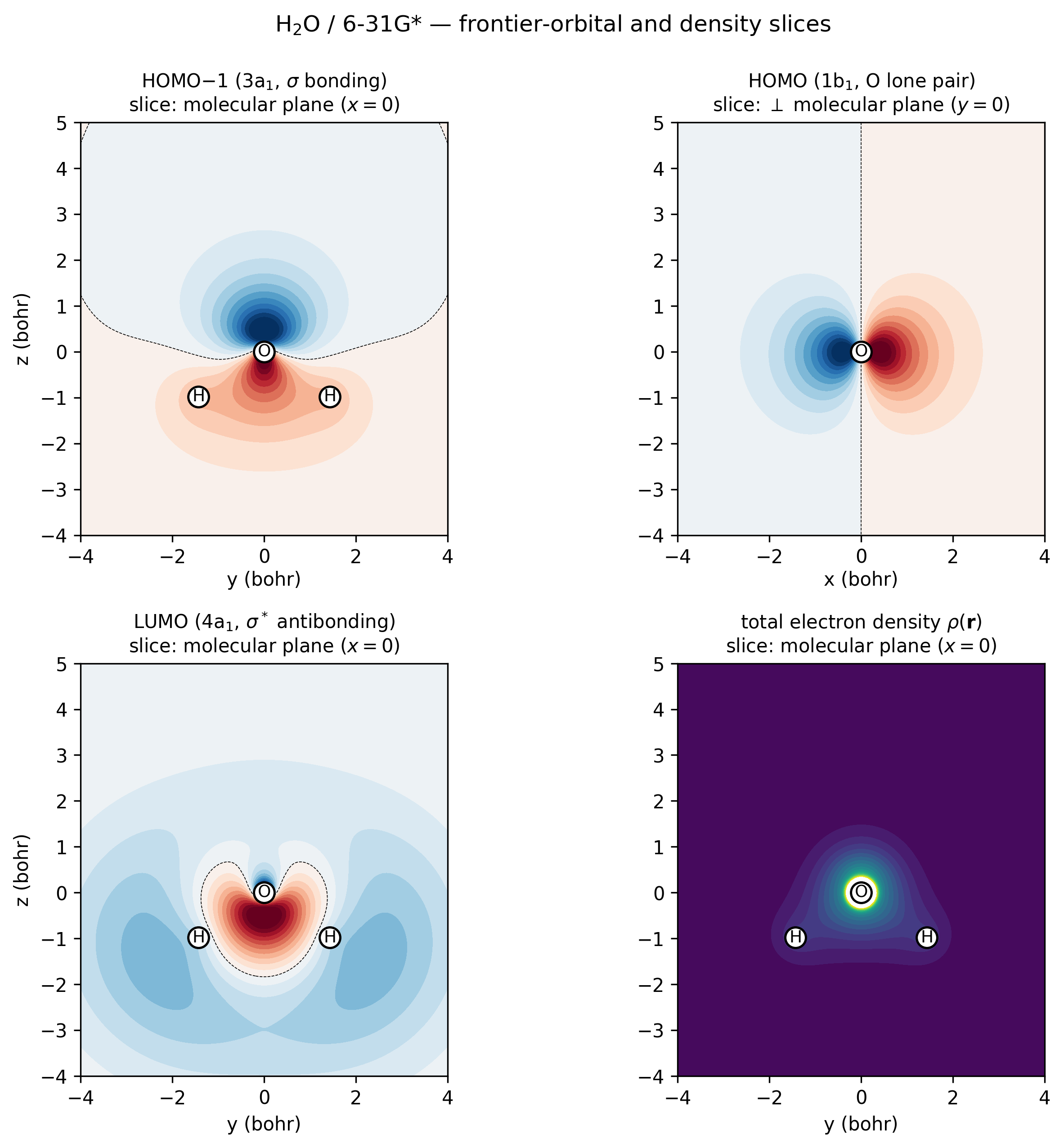
Four-panel contour plot of HOMO-1, HOMO, LUMO, and total density of water in the molecular plane and in a perpendicular slice through O. — H₂O / 6-31G* frontier orbitals and density, sampled directly via `vibeqc.evaluate_ao` and rendered as 2D contour slices. **Top-left** (3a₁ HOMO−1, \(\sigma\)-bonding): in-phase combination of the two O–H bonds with positive amplitude all along both bonds — the “valence σ” of water. **Top-right** (1b₁ HOMO, oxygen lone pair): the orbital is *perpendicular* to the molecular plane, so this slice goes through O at \(y = 0\) and shows the textbook two-lobe ±x dumbbell. **Bottom-left** (4a₁ LUMO, \(\sigma^*\)-antibonding): nodal plane between O and the H–H midpoint, lobes pointing away from H atoms. **Bottom-right** (total density): cusps at every nucleus and the smooth bonding ridge between O and each H. Regenerated by `examples/plots/water-frontier-orbitals.py`.¶

The 2D-slice route uses the same AO evaluator that write_cube_* uses internally, so the numbers are bit-identical to a thin slice through the cube file — but you skip the disk-write / external-tool round-trip when all you want is a sanity check.

Caveats¶

HF orbitals aren’t “truth”. Molecular orbitals are a representation-dependent quantity — Kohn-Sham orbitals from the same basis set often look visibly different. When comparing to the literature, note the method that generated them.
Phase arbitrariness. The overall sign of an MO is arbitrary — two SCF runs can land on C_i → +C_i or −C_i. The density is the physical quantity; the color of HOMO lobes can flip between runs.
Tighter basis → more structure. Minimal-basis HOMOs look bland; by TZVP you start seeing polarization lobes that are genuinely chemically informative.

Theory¶

What an “orbital isosurface” actually plots¶

A molecular orbital \(\phi_i(\mathbf{r}) = \sum_\mu C_{\mu i} \chi_\mu(\mathbf{r})\) is a real-valued function of \(\mathbf{r}\) in three-dimensional space (imaginary for k-space bands; see tutorial 12 for those). What viewers call an “isosurface at value \(c\)” is the mathematical surface

\[ \{ \mathbf{r} : \phi_i(\mathbf{r}) = c \} \]

rendered as a triangulated mesh. The marching-cubes algorithm (Lorensen-Cline 1987) converts the scalar field on a regular grid into this mesh; every mainstream viewer (VMD, PyMOL, Avogadro, ParaView) uses it or a close variant.

Common rendering conventions:

Color the two signs differently. Since \(\phi\) is real but signed, isosurfaces at \(+c\) and \(-c\) exist simultaneously. Showing both in complementary colors (cyan / orange, red / blue) makes the nodal structure visible.
Isovalue choice. \(c = 0.05\) bohr⁻³ᐟ² is a good default that captures the bonding lobes without drowning in the diffuse tail. Tighten to 0.08 for a compact view of valence MOs; loosen to 0.02 to see Rydberg-like tails.
The density \(\rho(\mathbf{r}) = \sum_i |\phi_i|^2\) is always positive and sign-ambiguous — an isosurface at \(\rho = 0.01\) shows electron localisation without the phase-flip artefact.

The Gaussian cube format¶

The cube writer samples the scalar field on a regular Cartesian grid and writes a plain-ASCII file. The structure:

Comment line 1
Comment line 2
  n_atoms   x0  y0  z0        <- origin of the grid (bohr)
  n_x       dx  0   0         <- grid vectors (bohr), direction and spacing
  n_y       0   dy  0
  n_z       0   0   dz
  Z_1   Q_1   x_1  y_1  z_1   <- atoms: atomic number, nuclear charge, position
  ...
  <floating-point values, in scanline order>

vibe-qc’s write_cube_mo evaluates \(\phi_i(\mathbf{r}_g)\) at every grid point \(\mathbf{r}_g\) by direct AO evaluation on the grid (uses the same evaluate_ao machinery that the DFT XC grid does internally) followed by the AO-to-MO contraction \(\phi_i(\mathbf{r}_g) = \sum_\mu C_{\mu i} \chi_\mu(\mathbf{r}_g)\). The write_cube_density path contracts against the density matrix instead: \(\rho(\mathbf{r}_g) = \sum_{\mu\nu} P_{\mu\nu} \chi_\mu(\mathbf{r}_g) \chi_\nu(\mathbf{r}_g)\).

Grid cost¶

File size scales as \(1 / \text{spacing}^3\). At 0.2 bohr on a water molecule with 3 bohr padding, that’s \(\sim 40^3 \approx 6 \times 10^4\) values; at 0.1 bohr, \(\sim 5 \times 10^5\). AO evaluation cost scales linearly in grid points and quadratically in basis functions, so doubling the resolution makes the file 8× bigger and the write 8× slower. Use 0.2 for quick looks, 0.1 for papers.

The sign-arbitrariness caveat¶

A single-reference SCF converges to a Slater determinant whose columns \(\mathbf{C}_i\) are eigenvectors of \(\mathbf{F}\). Eigenvectors are defined only up to a sign (real) or phase (complex), so the overall sign of an MO plotted on different SCF runs can flip. The density is invariant — \(|\phi_i|^2\) is well-defined — but the colored lobes of a rendered MO can swap between runs. When comparing MO pictures across codes, or across functionals, don’t chase the lobe-color pattern; chase the nodal structure.

Resources¶

~250 MB peak RAM, ~3 s on one core (Apple M2 baseline) for the H₂O / 6-31G* HF + cube-write at 0.2 bohr spacing. Cube-file size scales as \(1/\text{spacing}^3\); the AO evaluation on the grid scales linearly in grid points and quadratically in basis size, so dropping to 0.1 bohr makes the file 8× bigger and the write 8× slower.

References¶

Marching cubes. W. E. Lorensen and H. E. Cline, “Marching cubes: a high resolution 3D surface construction algorithm,” ACM SIGGRAPH Comput. Graph. 21, 163 (1987). The basis of every isosurface renderer in chemistry.
Gaussian cube file format. Defined informally in the Gaussian programme’s documentation; community-standardised description at https://paulbourke.net/dataformats/cube/ and the cubegen section of the Gaussian manual. vibe-qc’s writer matches the conventions Avogadro / VMD / PyMOL all consume.
Textbook treatment of MO visualization. W. J. Hehre, L. Radom, P. V. R. Schleyer, and J. A. Pople, Ab Initio Molecular Orbital Theory, Wiley (1986) — foundational MO pictures of organic molecules that set the conventions still in use.

Next¶

For periodic systems, XSF files play the role cube files do for molecules — see the volumetric-data user guide for the periodic equivalents (write_xsf_volume, write_bxsf for Fermi surfaces).