vibe-view: interactive viewer¶
vibe-view is a GPU-accelerated browser-based viewer for vibe-qc’s
QVF (.qvf) output archives. It reads the
zip + JSON manifest format produced by run_job(..., output_qvf=True)
and renders every section the calculation produced: structure,
electron density, molecular orbitals, band structures, spectra,
geometry-optimisation trajectories, vibrational modes, NEB / IRC
reaction paths, and more.
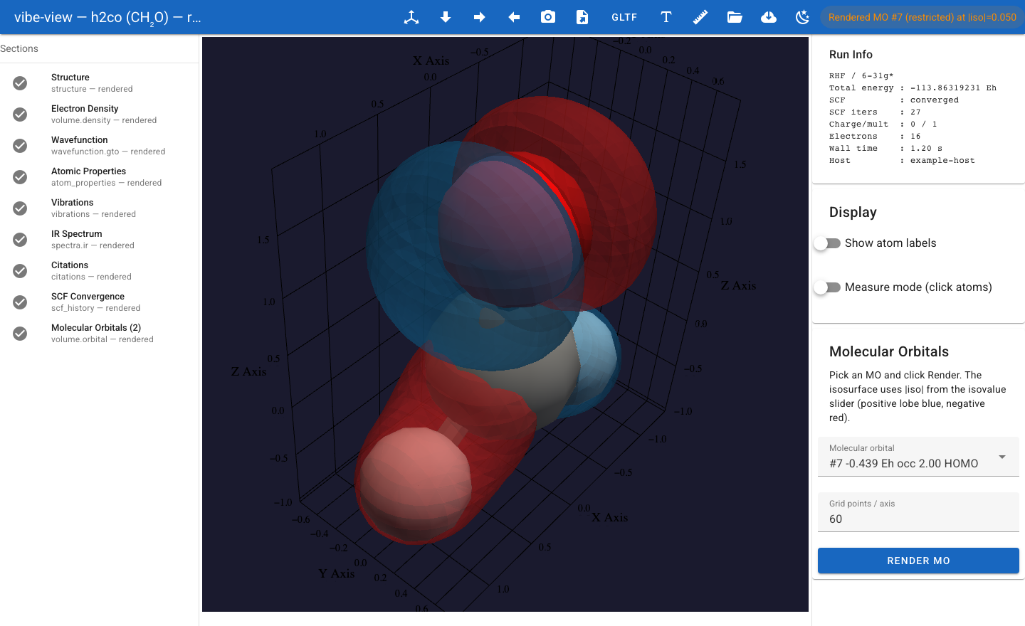
vibe-view in the browser: the section sidebar (left), the GPU-accelerated 3D viewport (centre), and per-section controls (right). Here, a molecular orbital with both signed lobes.¶
What you need on disk¶
Two things:
A
.qvffile produced by vibe-qc. Passoutput_qvf=Truetorun_joborrun_periodic_joband a{stem}.qvflands next to{stem}.out.vibe-view installed (it is a peer subproject under
vibe-view/inside the vibe-qc checkout, with its ownpyproject.toml).
Install¶
vibe-view is a co-located peer package, not a built-in part of
vibeqc. Two install routes:
# uv (vibe-qc's stated installer), from a vibe-qc checkout. Installs
# both vibe-qc and vibe-view in one step via the [tool.uv.sources] entry.
uv pip install -e '.[viewer-gpu]'

# With pip, the [viewer-gpu] extra can NOT pull vibe-view (pip ignores
# [tool.uv.sources]), so install vibe-view as a second step. The
# interactive viewer needs the [viewer] extra (trame); headless
# screenshot capture and QVF reading do not.
pip install -e .
pip install -e 'vibe-view/[viewer]'      # interactive viewer: vibe-view open
# capture-only / headless host (docs artifacts, CI, queue jobs):
#   pip install -e vibe-view/
The dependency footprint is pure-pip. The core install (QVF reading plus
headless screenshot capture) is PyVista, VTK, matplotlib, Plotly, Click,
Pydantic, and jsonschema. The interactive web viewer adds Trame and
uvicorn via the [viewer] extra. No conda, no JavaScript build step, no
npm. The heaviest single dep is VTK (about a 200 MB wheel), so the first
install takes a minute or two.
Verify the install:
vibe-view --version
# vibe-view 2.1.0.dev0  -- Roothaan's Roadrunner
Produce a .qvf file from vibe-qc¶
Pass output_qvf=True to either runner. The flag stacks freely with
write_density, write_molden_file, and the other artefact
toggles.
Molecular: H2O / PBE / 6-31G*¶
from vibeqc import Atom, Molecule, run_job

mol = Molecule([
    Atom(8, [0.0,  0.00,  0.00]),
    Atom(1, [0.0,  1.43, -0.98]),
    Atom(1, [0.0, -1.43, -0.98]),
])

run_job(
    mol,
    basis="6-31g*",
    method="rks",
    functional="PBE",
    optimize=True,                  # writes a geometry trajectory
    output="water",
    output_qvf=True,                # produces water.qvf
    write_density=True,             # embeds the SCF density isosurface
    write_molden_file=True,         # embeds wavefunction.gto + MOs
)
Produces water.qvf alongside the usual water.out / water.molden
/ water.traj / water.bibtex siblings.
Periodic: MgO rocksalt / RHF / sto-3g¶
import numpy as np
import vibeqc as vq

a = 4.21 / 0.529177                                    # Angstrom to bohr
mgo = vq.PeriodicSystem(
    3,
    np.eye(3) * a,
    [vq.Atom(12, [0.0, 0.0, 0.0]),
     vq.Atom(8,  [a/2, a/2, a/2])],
)
basis = vq.BasisSet(mgo.unit_cell_molecule(), "sto-3g")

kpath = vq.kpath_from_segments(
    mgo,
    segments=[
        ([0.0, 0.0, 0.0], "G", [0.5, 0.0, 0.5], "X"),
        ([0.5, 0.0, 0.5], "X", [0.5, 0.5, 0.5], "L"),
        ([0.5, 0.5, 0.5], "L", [0.0, 0.0, 0.0], "G"),
    ],
    points_per_segment=20,
)

vq.run_periodic_job(
    mgo,
    basis=basis,
    method="RHF",
    output="mgo",
    output_qvf=True,
    write_density=True,
    band_structure=vq.band_structure_hcore(mgo, basis, kpath),
)
The optional band_structure= kwarg embeds a band-structure section
in the archive so vibe-view can render the interactive Plotly band plot
without having to re-diagonalise.
Launch¶
Command line¶
vibe-view open water.qvf
Boots the Trame server on http://127.0.0.1:8080 and opens the
default browser at that URL. Flags:
vibe-view open water.qvf --port 9876        # bind to a different port
vibe-view open water.qvf --no-browser       # skip the auto-open
vibe-view open water.qvf --host 0.0.0.0     # bind to all interfaces (remote use)
Programmatic¶
from vibeview import launch_qvf

launch_qvf("water.qvf")                          # path on disk
launch_qvf(open("water.qvf", "rb"))              # any seekable file-like
launch_qvf(io.BytesIO(qvf_bytes), open_browser=False)  # in-memory
launch_qvf blocks until the Trame server stops (Ctrl+C). Pass an
already-constructed QVFReader instance if you want to inspect the
archive before launching the UI.
The UI¶
When the browser opens you get three regions:
Top bar: the source banner (program, version, calculation name) and the section-status pill.
Sidebar (left): the section tree. Click a section to make it the active section (loads its binary data on first click). Active sections drive the main viewport.
Viewport (centre): 3D scene for structure / volume / vibrations / trajectory sections; interactive Plotly chart for bands / spectra; table for
atom_propertiesandscf_history.
Comparing multiple files¶
Open several archives at once (vibe-view open a.qvf b.qvf ...); a Files
dropdown in the top bar switches the active file. With more than one open, a
Compare Files card appears in the right panel: the Overlay all structures
switch draws every loaded structure together in one viewport, one translucent
colour per file, with a colour-keyed legend of file names. This is handy for
seeing how a geometry shifts between two relaxations, methods, or polymorphs.
Structures are shown at their stored coordinates; toggle Align (RMSD fit to
first file) to Kabsch-superpose each onto the first file (when the atom counts
match), with the per-file RMSD to that reference shown in the legend. Clicking
any section exits compare mode.
For two files that both carry a volume.density section on the same grid, the
Density Difference card renders ρ_A − ρ_B as a two-colour isosurface (red =
accumulation where A > B, blue = depletion) over file A’s structure, handy for
deformation densities or before/after-adsorption maps.
Structure section¶
Atoms are drawn as CPK spheres with element-coloured surfaces and
the standard van-der-Waals radii. Bonds come from the explicit
bonds section if the producer wrote one; otherwise vibe-view
infers them from covalent radii. Crystals show the unit-cell
wireframe.
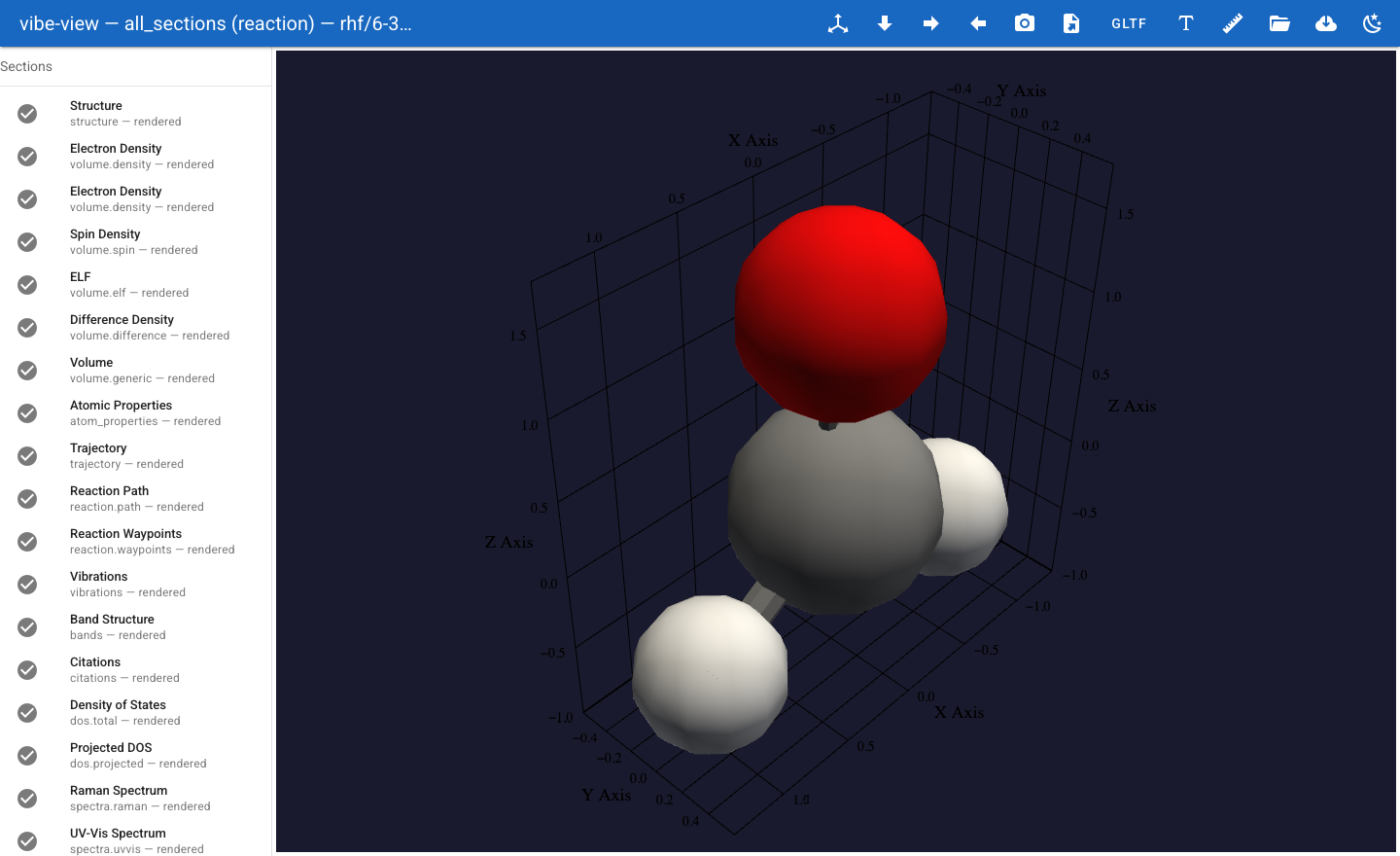
The structure panel — CPK spheres (Jmol colours, Z ≤ 96), inferred or explicit bonds, and the unit-cell wireframe for crystals.¶
Sidebar controls:
Replication (periodic only): set Nx, Ny, Nz to replicate the cell along the lattice vectors. Atoms, isosurfaces, and the cell wireframe all expand in lock-step.
Atom radii / colours: choose between CPK (default), van der Waals, and unit-radius schemes.
Building & editing (edit mode)¶
Press e (or the pencil icon in the top bar) to toggle edit
mode on the structure section. Click an atom to select it, click
empty space to place an atom of the element chosen in the Atom
Editor card; the card also changes the element of the selection,
deletes it, inserts fragments (methyl, hydroxyl, phenyl, …),
saturates open valences with hydrogens, and offers undo/redo
(Ctrl-Z / Ctrl-Y). Edits compound in place; Export vibe-qc
input (.py) and vq submission always use the geometry as edited.
Auto-optimize (Atom Editor card): while on, every edit pause relaxes the sketch in the background in a separate subprocess, streaming each optimizer step into the viewport so the atoms ease toward the relaxed geometry. The status line under the switch shows the running step / energy / max gradient, then
relaxed in N steps. Editing again mid-relax cancels and reschedules; one undo entry per relax run returns to the sketch as drawn. Needsvibeqcimportable in the viewer’s environment: when it isn’t, the switch snaps back off with the reason, and the viewer works exactly as before. Structures beyond 80 atoms are skipped to keep the background evaluations interactive.Auto-optimize engines: the default is vibe-qc’s MSINDO semi-empirical model (analytic gradients, elements H through Xe). When vibe-qc’s
[mace]extra is installed (PyTorch stack, Python 3.13 or older), an Engine picker appears offering MACE (the MIT-licensed MACE-MPA-0 foundation model, CPU): often better geometries, heavier per step, and the first use downloads the model weights (the status line says so). MACE energies are the model’s reference-shifted DFT-surface values, not vibe-qc total energies; MACE also ignores charge and spin. The ASL-gated academic MACE models are not offered here.
volume.density, volume.orbital, volume.spin, volume.elf, volume.difference, volume.generic, volume.potential¶
All volume kinds drive the same renderer: VTK marching cubes over
the grid .dat payload, producing an isosurface at the
configurable isovalue. Sidebar controls:
Isovalue: slider over the volume’s data range (default from
viewer_defaults, falling back to a kind-specific heuristic: 0.05 e/bohr^3 for densities, 0.04 bohr^(-3/2) for MOs).Colour map (signed-volume kinds):
volume.orbital,volume.spin,volume.difference, andvolume.potential(the electrostatic potential, signed in hartree/e) get a divergent map so the +/- lobes show in different colours.Opacity: 0 to 1 alpha.
Volume .dat blobs are lazy-loaded: nothing is read from the
zip until you activate the section. Large MO grids stay on disk
until you click them.
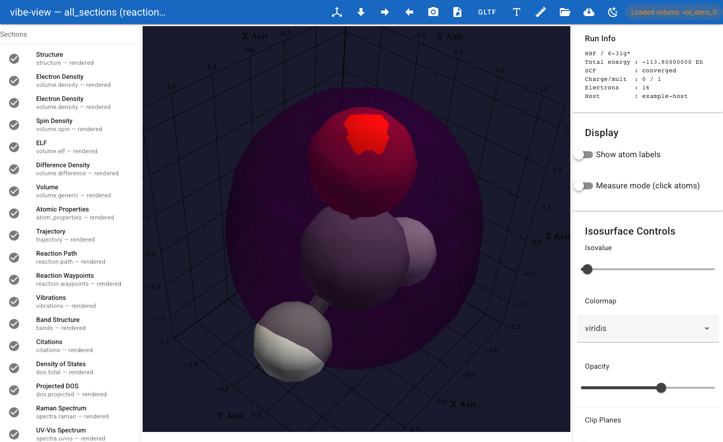
A scalar-field isosurface (electron density) from VTK marching cubes, drawn translucent over the structure. Signed fields — orbitals, spin, and difference densities — render both ± lobes in contrasting colours.¶
volume.rdg (NCI analysis)¶
Non-covalent interaction (NCI) surface. vibe-view contours the reduced density
gradient s(r) at the standard isovalue (0.3) and colours the surface by
sign(λ₂)ρ (the second Hessian eigenvalue of the density times ρ), computed from
a co-present volume.density section. Colour convention: blue = attractive
(e.g. H-bonds), green = van der Waals, red = repulsive/steric, clamped to ±0.05
a.u. With no density section in the archive the RDG surface renders uncolored.
Method: Johnson et al., JACS 132, 6498 (2010); NCIPLOT conventions,
Contreras-García et al., JCTC 7, 625 (2011).
bands¶
Interactive Plotly plot of every band along the k-path. The Fermi
level (from the bands.fermi field) is drawn as a horizontal
reference line. Hover any band to see its energy in eV at that
k-point. Energies are stored in eV in QVF v1 (see
QVF spatial and energy units).
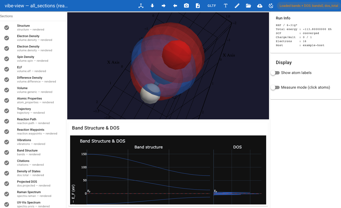
The band structure and, when a dos.total section is also present, the
density of states — drawn as one figure on a shared, Fermi-referenced
energy axis.¶
phonon_bands, phonon_dos¶
Lattice-dynamics panels for periodic systems. phonon_bands plots the
phonon dispersion (frequency along the Brillouin-zone q-path); phonon_dos
plots the phonon density of states. Both use cm⁻¹ on the frequency axis and
share the same 2D side panel as the electronic bands/DOS. Soft (imaginary)
modes are drawn below the zero-frequency line rather than hidden, so a
dynamical instability is visible at a glance. vibe-view plots the
producer-computed frequencies directly; cite your phonon method on the
producer side.
equation_of_state¶
Volume-energy panel. The sampled (V, E) points are plotted as markers; the
producer’s fitted curve (3rd-order Birch-Murnaghan or Murnaghan, per
fit.model) is overlaid by evaluating the published energy form at the fitted
V0/E0/B0/B0’, and the equilibrium volume V0 is marked. The fitted bulk modulus
B0, B0’, and the model reference (e.g. Birch 1947) are annotated in the panel.
Units follow spec §4.14 (Angstrom³ volumes, eV energies, GPa bulk modulus).
fermi_surface¶
Fermi surface in reciprocal space (Å⁻¹). For each band near E_F the archive
stores E(k) − E_F on a γ-centered Monkhorst-Pack mesh; vibe-view builds the
reciprocal lattice from the real-space lattice_vectors and contours each band
at E = E_F, drawing one sheet per band (distinct colours) inside the
reciprocal-cell wireframe. Because this is k-space rather than real space, the
molecular structure is hidden while the Fermi surface is shown; click any
real-space section to bring the structure back. When more than one band crosses
E_F, a Fermi Surface Bands multi-select in the right panel toggles which
sheets are drawn, so an individual sheet can be isolated. Spec §4.12.
spectra.ir, spectra.uvvis, spectra.raman, spectra.ecd, spectra.vcd, spectra.nmr, spectra.generic¶
Each spectrum renders as a Plotly stem chart of intensities vs frequency, with hover tooltips showing the per-peak metadata. The x-axis unit follows the spectrum kind (cm^-1 for IR / Raman, eV for UV-Vis, ppm for NMR).
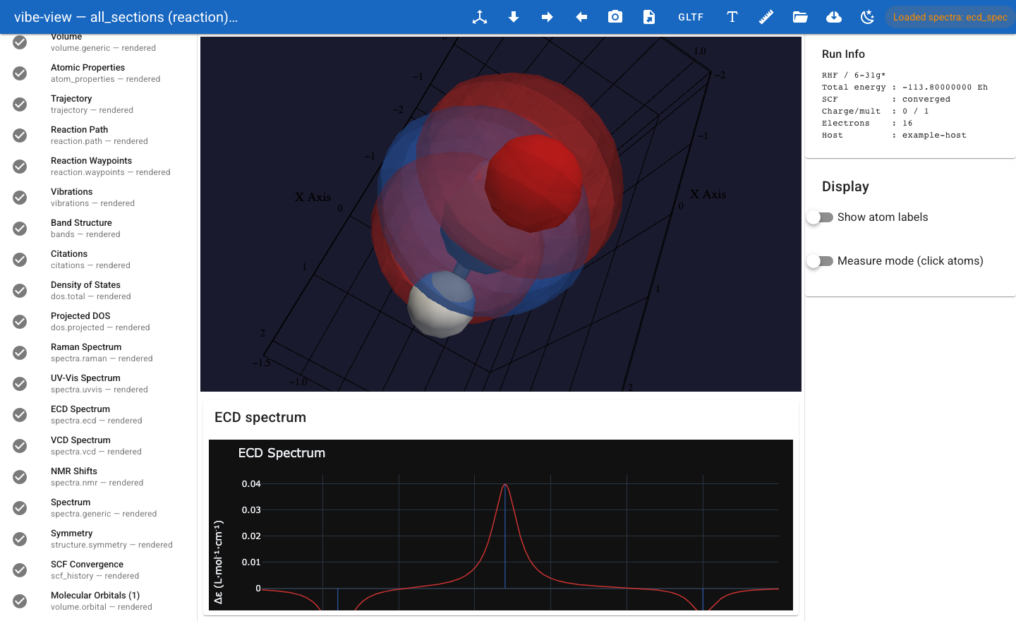
A 1-D spectrum (ECD shown) as a Plotly chart with hover tooltips. Signed spectra (ECD / VCD) keep their negative Cotton bands.¶
trajectory and reaction.path¶
Frame-by-frame animation with a play / pause / step button strip
underneath the viewport. Bonds are inferred per-frame from
covalent radii so they update with the geometry. A small energy
chart above the timeline plots metadata.energies vs frame index
for geometry-optimisation runs.
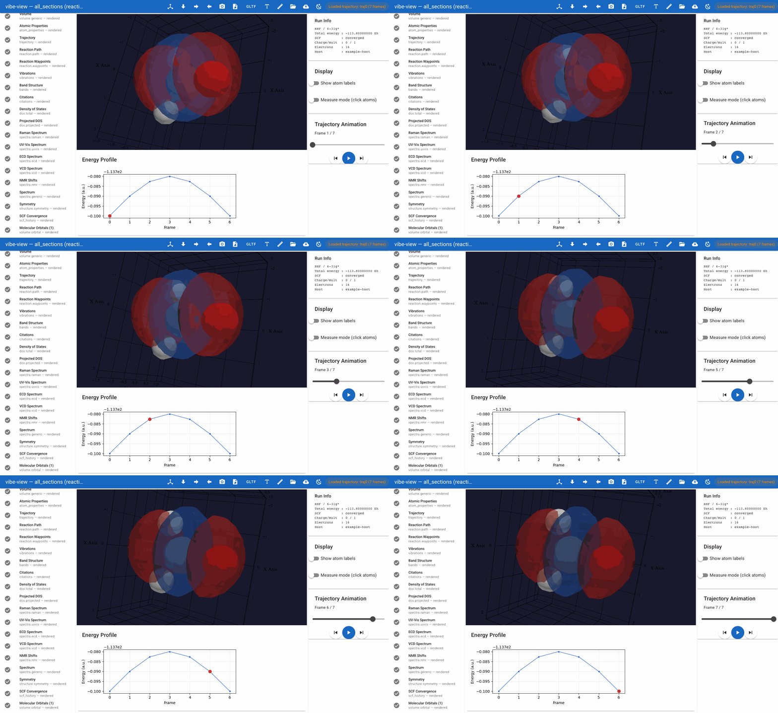
Frame-by-frame trajectory playback; the play / pause / step strip drives the timeline and the energy chart tracks the current frame.¶
reaction.path has the same binary layout as trajectory but
additionally renders waypoint markers (reactant / TS / intermediate
/ product) on the timeline.
Periodic reaction paths. When the frames are
PeriodicSystem instances (slabs, surfaces, periodic NEB
trajectories), the archive carries the per-frame lattice +
dimensionality so the renderer can draw the unit cell and
(eventually) wrap atoms across periodic boundaries. It stays
qvf_version: 1: a consumer detects a periodic reaction path by
the lattice member’s presence, not by a version number.
The schema additions are minimal: an optional
lattice binary member on the reaction.path section
(columns = a, b, c, in bohr, matching
vibeqc.PeriodicSystem.lattice) plus a dim integer in the
metadata JSON. A shared lattice across all frames stores once as
shape [3, 3]; per-frame lattices store as [n_frames, 3, 3]
(forward-compat with variable-cell scans). Molecular reaction paths
keep emitting v1 archives, there is no migration to do. See
python/vibeqc/output/formats/qvf_manifest_v2.schema.json for
the canonical v2 contract; the writer detects periodic frames
automatically and bumps the archive version.
Rendering (Increment B). When a v2 periodic reaction.path
is activated, vibe-view draws the unit-cell wireframe in the 3D
scene (the same parallelepiped style the structure renderer
uses) and wraps every frame’s atom positions into the central
cell along the first dim lattice vectors. For a slab
(dim=2) that means a + b are wrapped while the non-physical
direction c stays open, an adsorbate that climbs above the
surface keeps climbing in the scene instead of jumping back to
the bottom of the cell. The wrap is naive modulo-1 on
fractional coords; frame-to-frame continuity is not anchored
across cell crossings (atoms can flip from one boundary to the
opposite mid-animation in pathological cases, chemistry NEBs
typically stay within the central cell, so this is rare in
practice). Variable-cell paths ([n_frames, 3, 3] lattices)
re-emit the box per frame, so the cell animates with the
geometry.
vibrations¶
Mode-selector dropdown to pick the normal mode (sorted by frequency); the structure animates with the displacement vector applied sinusoidally. Frequencies are in cm^-1.
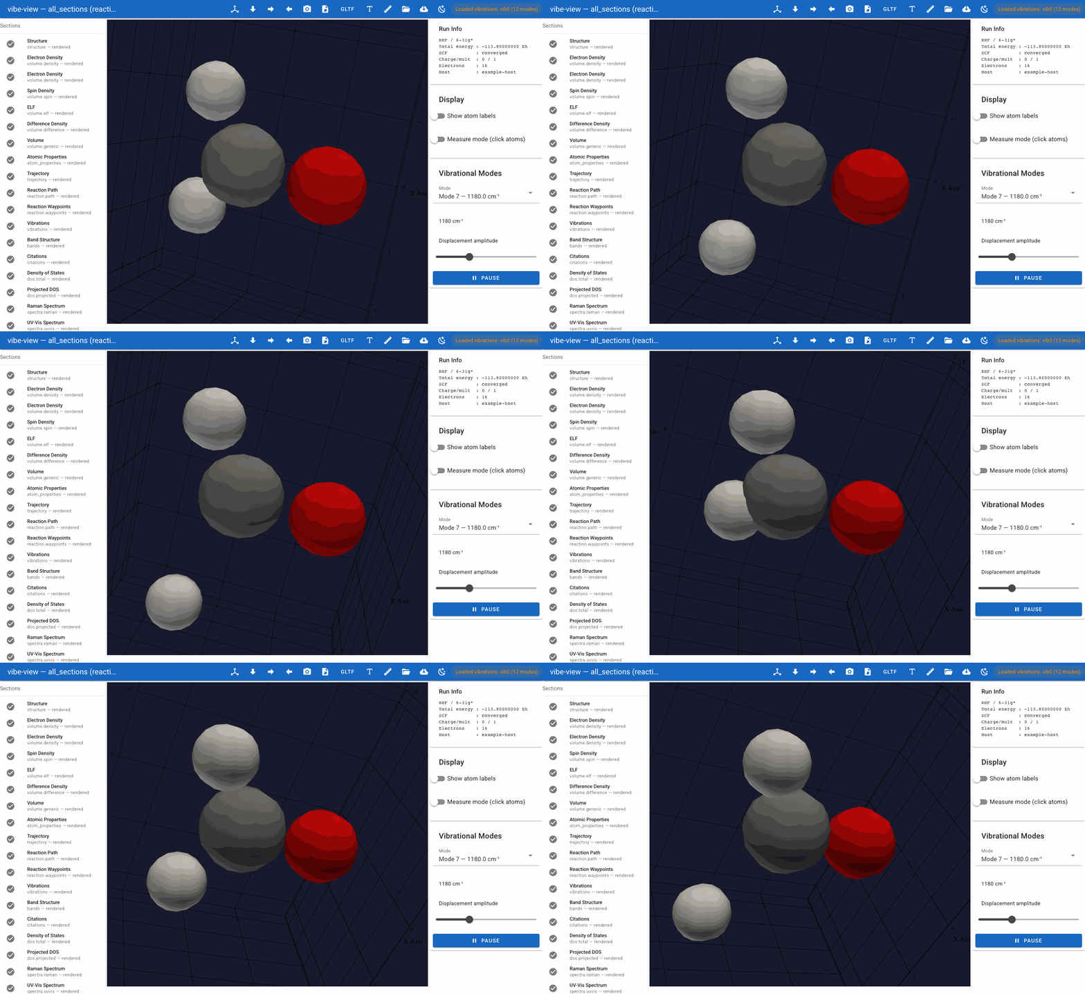
A normal mode animated about the equilibrium geometry. Mode labels
carry the IR intensity when a companion spectra.ir section is present.¶
atom_properties¶
Tabular display of mulliken_charge / loewdin_charge /
spin_population (whichever the producer wrote). Color-coded
per-atom highlighting in the 3D viewport.
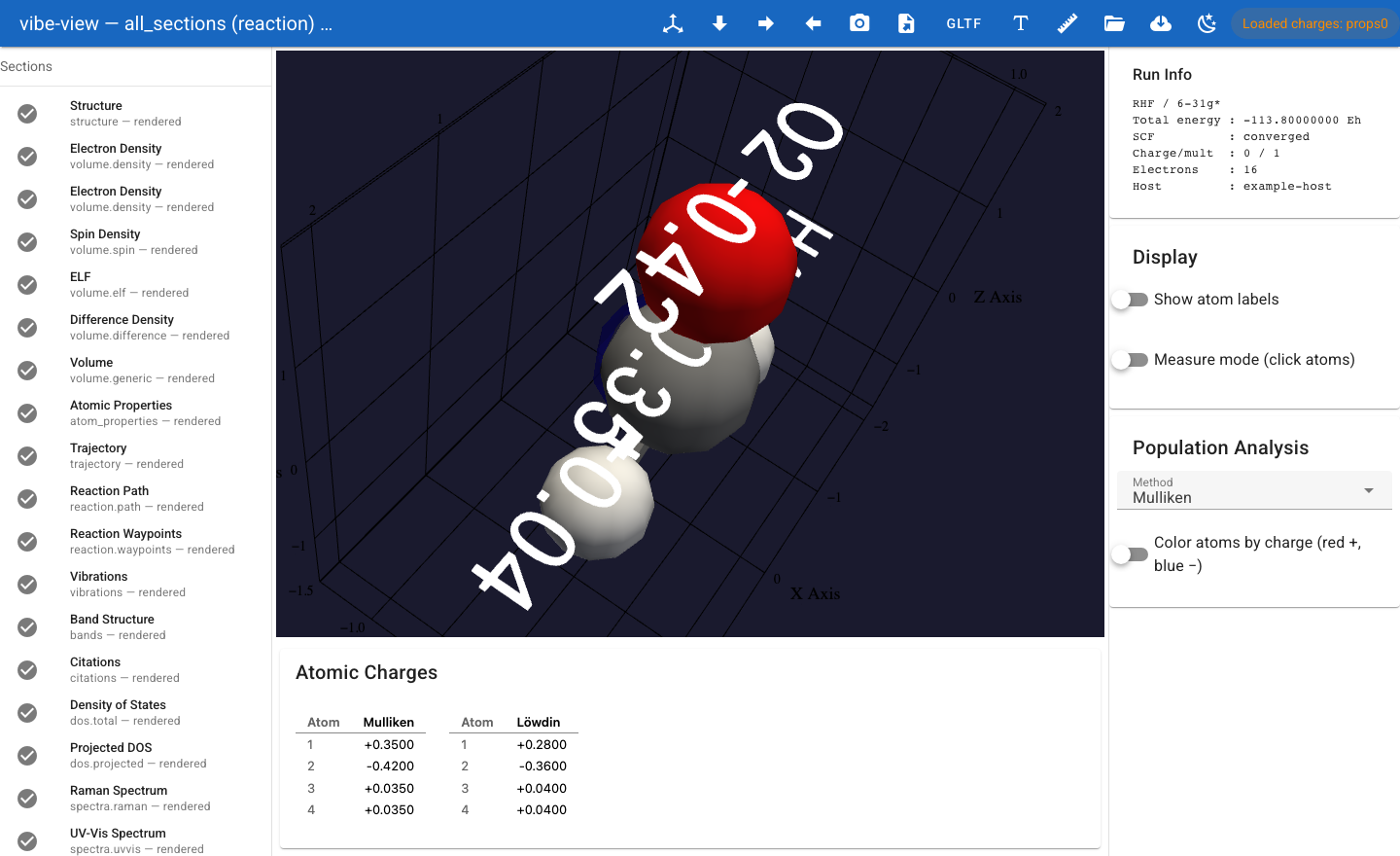
Atomic charges as a table plus a 3D overlay; “colour by charge” tints each atom (red positive, blue negative). On replicated periodic cells the tint follows every replica.¶
wavefunction.gto¶
Browse the molecular orbitals as a list (with energies and
occupations) and click any MO to render its isosurface. vibe-view
resamples the orbital from the embedded GTO basis + MO coefficients
on a grid of its own choosing, so you can inspect any MO without
the producer having to pre-evaluate it. Compute total density sums
the occupied MOs (ρ = Σ occ_i |ψ_i|²) on the fly into a density isosurface
without needing a stored volume.density section; the status reports
∫ρ dV as an electron-count check.
scf_history¶
Two-pane chart: energy vs iteration (top) and |DIIS error| vs
iteration (bottom). Hover any iteration to see the exact numbers.
structure.symmetry¶
Compact info panel with the spglib output: space group name, Hall number, international symbol, Wyckoff positions, equivalent atoms.
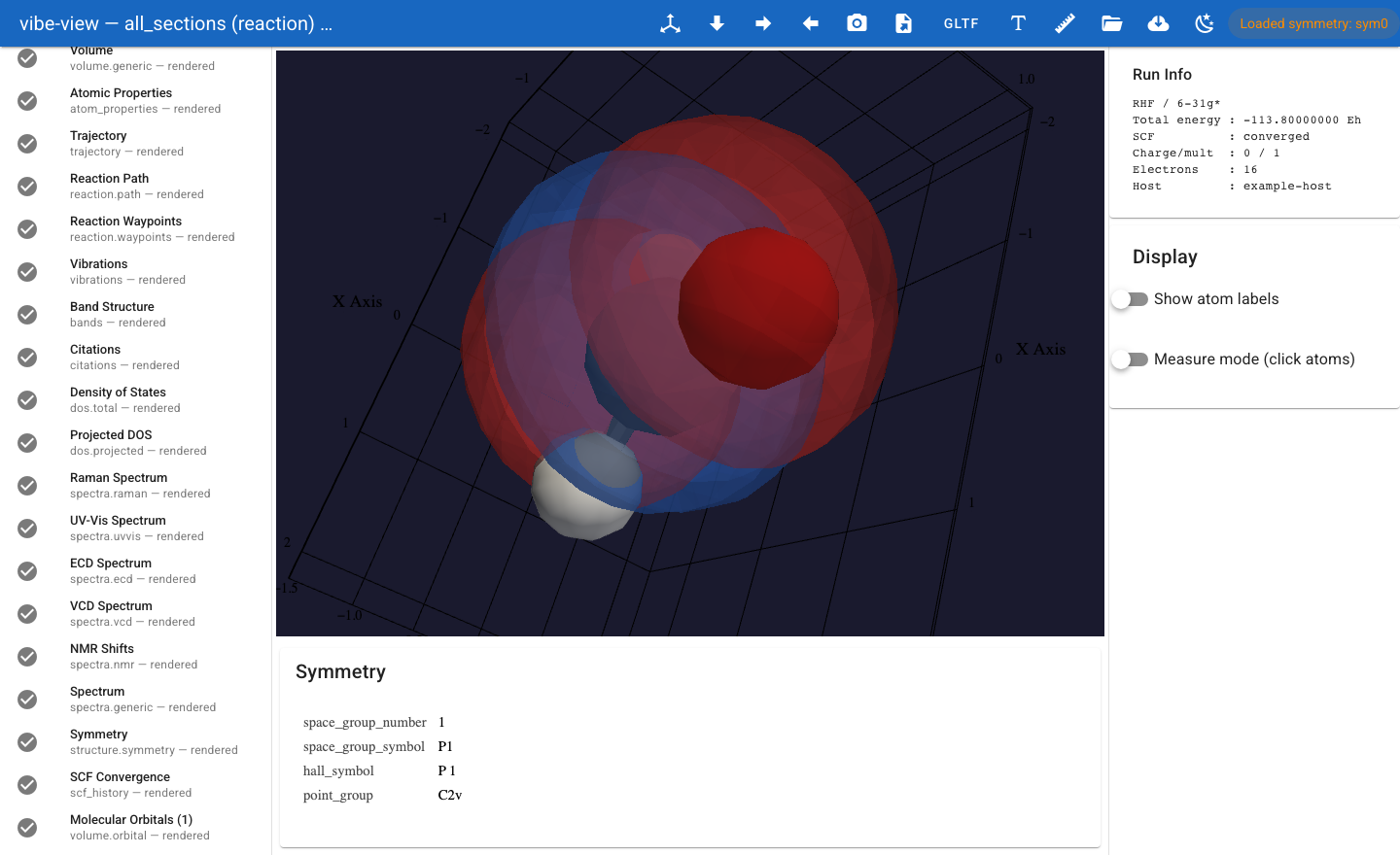
The symmetry panel surfaces every key spglib reports for the structure.¶
citations¶
The embedded BibTeX bundle is rendered as a copy-paste-friendly block. Pairs with the citations user guide: the viewer shows you what to cite, the producer wrote the database entries.
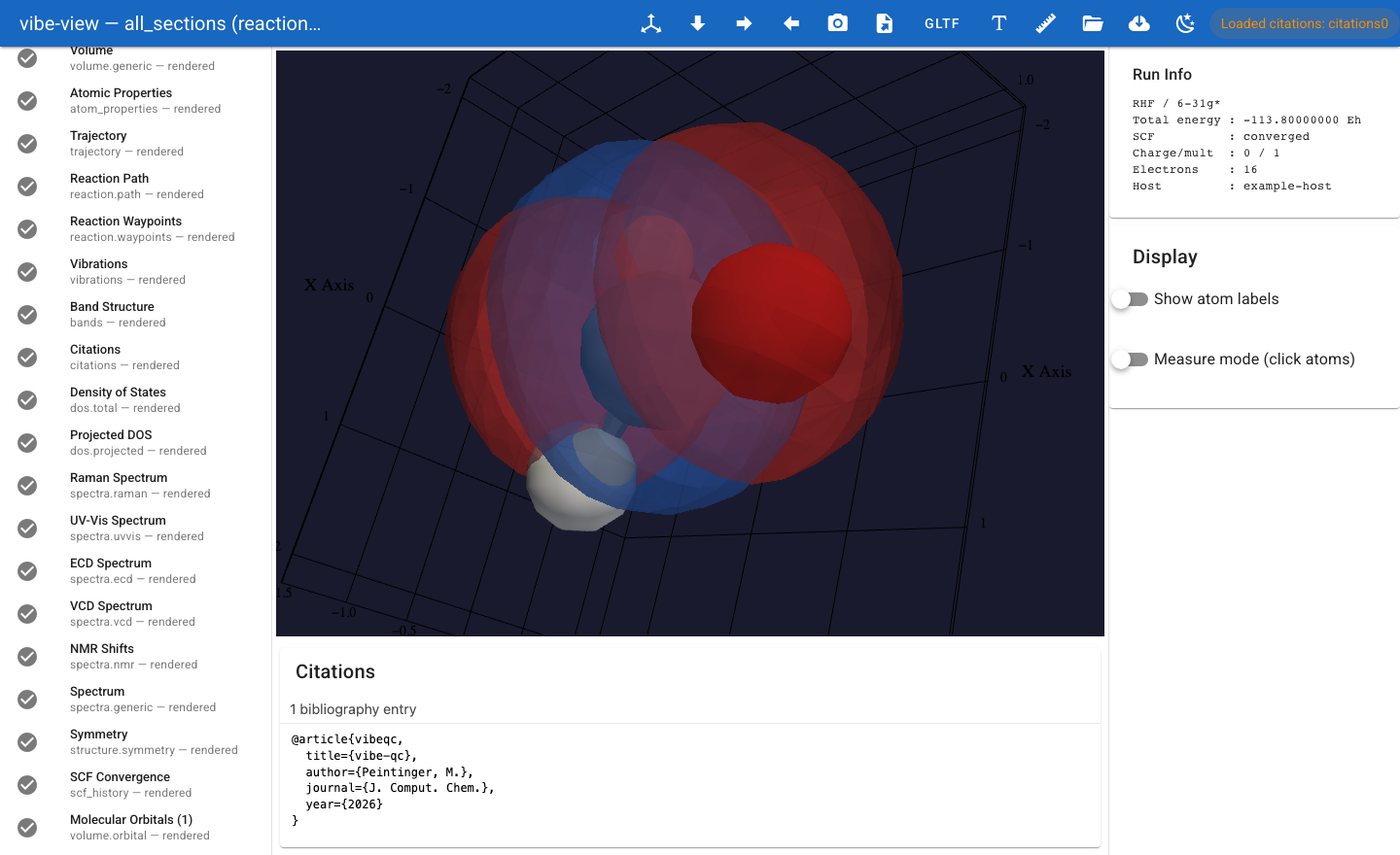
The citations panel renders the embedded BibTeX bundle as a copy-paste block.¶
Running and monitoring jobs (vq)¶
vibe-view is also a cockpit for the vibe-queue (vq) job runner, not
just a file viewer. Open the Job Manager from the server icon
(mdi-server-network) in the app bar. It lists the local vq queue,
tracks job state, and opens finished results straight into the viewer:
Each row shows a colour-coded state chip (
pendinggrey,runningblue,suspendedamber,completedgreen,failed/killed/interruptedred), the job name and short id, elapsed time, and an open action that fetches a completed job and loads its.qvffiles.A queue-overview strip summarizes the local queue at a glance: daemon health, host and
vqversion, capacity (max CPUs / concurrent jobs), and current load (running / pending CPUs).Live monitor (a switch) includes every state (queued, running, suspended) and auto-refreshes every 5 seconds, with a per-job status and stdout/stderr log tail so you can watch a job progress without leaving the viewer.
Submit from the viewer: the submit dialog generates a vibe-qc input script from the current structure and submits it through
vqwith a job name and tag.
Live reload¶
Flip Auto-reload on file change (the Display card in the left panel) and vibe-view watches the open file and hot-reloads it whenever its content changes. The watcher is content-based, not timestamp-based: it fingerprints the QVF manifest per section, waits for the file to settle, holds off on a half-written archive, and then reloads only what actually moved: the active panel alone for a change confined to a 2D-panel section, or the full scene (your camera preserved, the active section restored) for anything structural. If you are parked on the last frame of a growing trajectory, the reload keeps you on the head as new frames arrive.
Streaming a running job¶
A vibe-qc job started with checkpoint_qvf=... rewrites a live QVF
snapshot as it runs, carrying provenance.run_status, a monotonic
provenance.checkpoint, and partial on still-growing sections (see
the streaming section of the QVF reference).
vibe-view surfaces that stream:
In the Job Manager, a running job that has written a checkpoint shows a Watch live action (the eye icon). Clicking it opens the job’s checkpoint QVF and turns auto-reload on for you (no need to know the path). Jobs submitted from the viewer stream a checkpoint by default, so a job you just launched is immediately watchable.
An app-bar chip reflects the job status: it pulses running (with
#seq · iter N · E … Ehfrom the latest checkpoint), then settles green converged or red failed on the terminal snapshot, and the status bar announces the finish.A section the producer is still growing (an optimization
trajectory, SCF history mid-run) is badged streaming in the sidebar and reloads in place as it grows.
When run_status leaves running, the checkpoint you are already
watching is the settled result, so no separate fetch is needed.
Exporting animations to video¶
vibe-view animate renders an animatable section to MP4 (needs
ffmpeg on PATH) or GIF (needs only Pillow):
vibe-view animate opt.qvf                            # auto-detect the section
vibe-view animate neb.qvf --kind reaction            # NEB band: reactant -> TS -> product
vibe-view animate vib.qvf --kind vibration --mode 7  # one normal mode
vibe-view animate opt.qvf -k trajectory --fps 8 --format gif
--kind auto (the default) picks the first of trajectory,
reaction.path, vibrations, or wavefunction.gto it finds. The same
renderers are importable (render_trajectory_video,
render_reaction_video, render_vibration_video, and
render_orbital_animation in vibeview.animation), each returning the
output path (or None when the archive has no matching section):
from vibeview.qvf import QVFReader
from vibeview.animation import render_reaction_video

render_reaction_video(QVFReader("neb.qvf"), "neb.mp4", fps=5, format="mp4")
viewer_defaults: producer-side hints¶
The producer can suggest defaults to the viewer in the manifest
under viewer_defaults. vibe-view picks these up on load and
applies them before rendering anything.
write_qvf(
    "water.qvf",
    ...,
    viewer_defaults={
        "auto_open": ["density"],          # activate the density section by default
        "density": {                       # per-section render hints
            "isovalue": 0.04,
            "colormap": "viridis",
            "opacity": 0.55,
        },
        "bookmarks": [                     # camera bookmarks
            {"name": "front",  "camera": {...}},
            {"name": "above",  "camera": {...}},
        ],
    },
)
Hints are non-binding: the user can override any of them through the UI, and unknown viewer_defaults fields are ignored rather than rejected.
Supported kinds¶
The viewer’s renderer registry lives at
vibe-view/src/vibeview/kinds.py::SUPPORTED_KINDS. The full
writer / viewer support matrix is in the
QVF design doc § 4.
Anything not in the registry is classified as “skipped,
unsupported” by the viewer and listed in the banner. The viewer
never aborts on an unknown kind; it just leaves that sidebar entry
unclickable.
If you write a custom kind under the x_<vendor>.* namespace, the
viewer reports it as “skipped, vendor namespace” with the vendor
name extracted. To get a kind rendered, add it to
SUPPORTED_KINDS and wire a matching renderer under
vibe-view/src/vibeview/renderers/.
Common pitfalls¶
“vibe-view: command not found”¶
You installed vibeqc but not vibe-view. Install with one of the
routes above (uv pip install -e '.[viewer-gpu]', or under pip the
two-step pip install -e . && pip install -e vibe-view/). The viewer is a separate package
because its dependency footprint (VTK, PyVista, Trame) is large
and not every vibe-qc user wants it.
“ManifestValidationError”¶
The archive’s manifest.json does not satisfy the canonical JSON
Schema at python/vibeqc/output/formats/qvf_manifest.schema.json.
This usually means the producer is older than the viewer or vice
versa. Both sides load the same schema (vibe-view bundles it as a
symlink), so a sha256-identity test pins them; if the archive was
produced by a third party, ask them to validate with
validate_qvf before sharing.
“SHA256MismatchError”¶
A binary payload in the archive has a different sha256 than the manifest claims. Usually means the archive was edited after writing (zip-shuffled, copied truncated, …). The viewer reports this per-section: other sections still load.
“the browser opened but the page is blank”¶
Trame uses Vue 3 + WebSocket. A very strict ad-blocker or
corporate proxy can break the WebSocket handshake. Either
allow the page in the blocker, or launch with --host 0.0.0.0
and open the URL by hand from a different browser profile.
Firefox on macOS 15+ “Unable to connect to 127.0.0.1”¶
macOS 15 (Sequoia) added a system-level Local Network
permission gate that is denied to Firefox by default. The
symptom is unmistakable: Safari and Chrome connect to
http://127.0.0.1:8080 fine, but Firefox shows “Unable to
connect” with a hint about Local Network permissions in
macOS Privacy & Security. Two fixes:
Grant Firefox the permission. System Settings → Privacy & Security → Local Network → toggle Firefox on. Refresh the page. (vibe-view does not need elevated permissions itself; only the browser does.)
Or use a different browser. Safari and Chrome are unaffected because they were grandfathered into the permission system. Open
http://127.0.0.1:8080there while the vibe-view server keeps running in the terminal.
vibe-view itself binds to 127.0.0.1 only by default; nothing
on the server side needs reconfiguring. If you launched with
--host 0.0.0.0 for remote access the same Local Network
gate applies to any LAN browser hitting the box, not just
Firefox.
“vibe-view server starting on …” printed but the browser cannot connect for a few seconds¶
vibe-view announces “ready” only once uvicorn has actually
bound the TCP port (the watcher polls the listener in a
background thread, so the “ready” line and the automatic
browser-open happen post-bind). If you set --no-browser
and open the URL by hand immediately after launching, you
may still race the bind on slow machines; refresh once and
you should connect. If “ready” never appears, see the next
entry.
“vibe-view: warning, server did not bind within 10s”¶
uvicorn entered the asyncio main loop but never made it to binding the TCP socket. Two common causes:
Port already in use. Another process is bound to the same port (a stale vibe-view, an aborted SSH tunnel, Docker Desktop, …).
vibe-view opennow normally catches this before launch and aborts with a “port … is already in use” message instead (see the entry below); the 10 s warning only remains for the rarer case where the socket is held in a state the pre-check misses. Either way, pick a different port with--port 9876and retry, or find the offender:lsof -nP -iTCP:8080 -sTCP:LISTEN
uvicorn import-time failure. A missing dependency in the venv (the historical case was the now-fixed missing
uvicorndeclaration in vibe-view’s pyproject; reinstall if you see aModuleNotFoundErrorin the stderr just before the warning).
“vibe-view: port 8080 is already in use”¶
vibe-view open pre-checks the port and stops with this message
when something is already listening there, most often a vibe-view
you left running in another terminal (servers stay up until you
press Ctrl+C; they have no idle timeout). Stop the other server, or
start this one on a free port:
lsof -nP -iTCP:8080 -sTCP:LISTEN   # find what owns the port
pkill -f "vibe-view open"           # …or just stop stale vibe-view servers
vibe-view open water.qvf --port 8090
This guard exists because, before it, open would connect to the
existing listener, announce “ready”, and open your browser at the
stale server while the new one died unseen; see the next entry.
The viewer shows a structure but the mouse does nothing (can’t rotate / zoom)¶
Almost always a stale server, not a viewer bug; rotation, zoom, and pan work in Chrome, Safari, and Firefox. Because vibe-view servers run until Ctrl+C, a browser tab can outlive the server behind it (you stopped it, your machine slept, or you re-launched and the new process could not bind the busy port). The tab keeps showing the last rendered frame (the structure looks fine) but its WebSocket is gone, so nothing responds to the mouse. Start fresh and use the new tab:
pkill -f "vibe-view open"     # stop any stale servers
vibe-view open water.qvf       # interact with the tab this one opens
Programmatic API¶
vibe-view’s API is intentionally minimal. Most users want
launch_qvf:
from vibeview import launch_qvf, QVFReader, QVFOpenError

# One-line launch
launch_qvf("water.qvf")

# In-memory archive (no temp file). Pair with vibeqc.output.qvf_bytes
# for an end-to-end producer → viewer hand-off that never touches disk.
from vibeqc.output import qvf_bytes
data = qvf_bytes(plan, molecule=mol, result=scf_result, mo_data=mos)
launch_qvf(data)

# Inspect first, then launch
try:
    reader = QVFReader("water.qvf")
except QVFOpenError as e:
    print(f"bad archive: {e}")
else:
    print(reader.sections)             # list of Section objects
    print(reader.source.version)       # producer version
    launch_qvf(reader)                 # reuses the open reader
QVFReader accepts a path, raw zip bytes, or any seekable binary
file-like (BytesIO, opened file). It validates the manifest at
construction time and lazy-loads section payloads on demand.
The full reading-side API for callers who want to consume .qvf
archives outside vibe-view is in the
QVF consumer reference.
See also¶
QVF format design: the producer / consumer contract, manifest schema, per-section payload conventions.
QVF consumer reference: the reading-side Python API for callers that want to ingest
.qvfarchives without launching vibe-view.vibe-view walkthrough: short end-to-end example that runs a calc, opens the result in vibe-view, and walks through what each panel does.
moltui terminal viewer: the terminal-only sibling viewer for SSH / no-X11 environments.
Output files reference: the full family of artefacts vibe-qc emits alongside the
.qvf.Background, QVF v1 grows up: basis sets, full reactions, and a reference viewer (peintinger.com, May 2026): the post that introduced vibe-view, with its companion Quantum chemistry needs a modern file format.