Band structure and density of states¶

Band structure is to periodic systems what the MO diagram is to molecules, the ordered energy levels that tell you whether a crystal is a metal, semiconductor, or insulator, and what the gap is when it’s not metallic. vibe-qc samples the one-electron Hamiltonian on a k-path (for bands) or a k-mesh (for DOS), plus a matching matplotlib plotter for publication-style figures.

This tutorial uses the same 1D H2 molecular crystal from the periodic HF tutorial, two bands (bonding + antibonding), clear band-gap picture, tiny compute cost.

Minimum example¶

The script below builds the 1D H2 chain, defines a Γ → X k-path along the chain axis, and computes both the two-band Hcore band structure and a Gaussian-broadened density of states in a single pass:

import vibeqc as vq

# 1D H2 chain: unit cell = one H2 molecule (bond 1.4 bohr),
# lattice vector a = 6 bohr along x.
system = vq.PeriodicSystem(
    dim=1,
    lattice=[[6.0, 0.0, 0.0], [0.0, 30.0, 0.0], [0.0, 0.0, 30.0]],
    unit_cell=[vq.Atom(1, [0.0, 0.0, 0.0]),
               vq.Atom(1, [1.4, 0.0, 0.0])],
)
basis = vq.BasisSet(system.unit_cell_molecule(), "sto-3g")

# Γ → X along the chain axis: fractional k from (0,0,0) to (½,0,0).
kpath = vq.kpath_from_segments(
    system,
    [((0.0, 0.0, 0.0), "Γ", (0.5, 0.0, 0.0), "X")],
    points_per_segment=40,
)

bands = vq.band_structure_hcore(system, basis, kpath, n_electrons_per_cell=2)
dos   = vq.density_of_states_hcore(
    system, basis, mesh=[80, 1, 1],
    sigma=0.02, n_electrons_per_cell=2,
)

You now hold two convenience objects:

bands.energies, (n_kpoints, n_bands) numpy array (Hartree).
bands.e_fermi, the HOMO level (chemical potential at T=0).
dos.energies / dos.dos, Gaussian-broadened DOS on an auto-chosen energy grid.

At the edges:

Γ:  bonding = -2.6660 Ha,   antibonding = -1.8335 Ha
X:  bonding = -2.6542 Ha,   antibonding = -1.9638 Ha
Fermi level: -2.6542 Ha   (filled bonding band, empty antibonding)

The plot¶

One call to bands_dos_figure turns the bands and dos objects into the publication-style two-panel figure and writes it to disk:

from vibeqc.plot import bands_dos_figure

fig = bands_dos_figure(bands, dos, title="H2 chain (STO-3G, Hcore)")
fig.savefig("h_chain_bands.png", dpi=150)

You get a two-panel figure: bands on the left with high-symmetry labels (Γ, X) along the bottom, DOS on the right sharing the same energy axis, Fermi level marked in both panels as a horizontal line.

H₂ chain bands and DOS

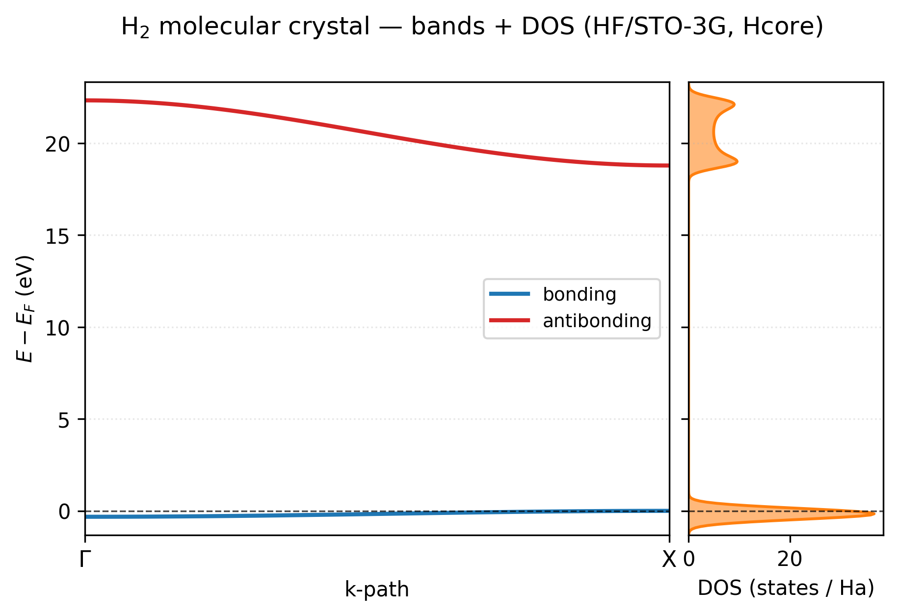
The two-band picture is exactly what s-orbital tight binding predicts. The bonding band (blue, just below \(E_F\)) is essentially flat, total bandwidth ~0.3 eV, because neighboring H₂ molecules are 3.2 bohr apart in this loose chain and their bonding orbitals barely overlap. The antibonding band (red, ~20 eV above) has a much wider dispersion (~3.5 eV) because the antibonding orbital has a node between the two H atoms of one molecule and lobes pointing toward the next molecule’s nucleus, so its energy is much more sensitive to the Bloch phase. The DOS panel makes both visible at a glance: a sharp tall peak at the Fermi level (the flat bonding band gives a near-singular DOS) and the broader two-peak structure of the dispersing antibonding band higher up. There’s clean empty space between the two, this is an insulator with an ~19 eV direct gap.

The figure is regenerated by [examples/plots/h-chain-bands-dos.py](https://gitlab.peintinger.com/mpei/vibeqc/-/blob/main/examples/plots/h-chain-bands-dos.py).

What the picture teaches¶

Two bands, as expected. STO-3G gives each H one s orbital; one H2 per cell = two AOs = two bands.
Bonding band is almost flat. Dispersion along Γ → X is only ~12 mHa = 0.3 eV, because neighboring H2 molecules (3.2 bohr apart) barely overlap their bonding orbitals.
Antibonding band disperses more (~130 mHa = 3.5 eV). The anti-bonding orbital has a node between H atoms of one molecule and constructive overlap with the nearest H of the next molecule, so its energy is more sensitive to the k-point.
There’s a gap everywhere, this is an insulator. Shrink the lattice parameter (a) and the antibonding band eventually crosses down below the bonding at Γ; at that point the system is a semimetal and HF refuses to converge, consistent with the Peierls-instability story from [examples/periodic/input-h-chain-peierls.py](https://gitlab.peintinger.com/mpei/vibeqc/-/blob/main/examples/periodic/input-h-chain-peierls.py).

The crystalline orbitals at Γ and X¶

The “almost-flat bonding band” and “wider antibonding band” claims are easier to see than to argue about. Below are the four crystalline orbitals at the two endpoints of the k-path, evaluated on a 2D slice through the chain plane:

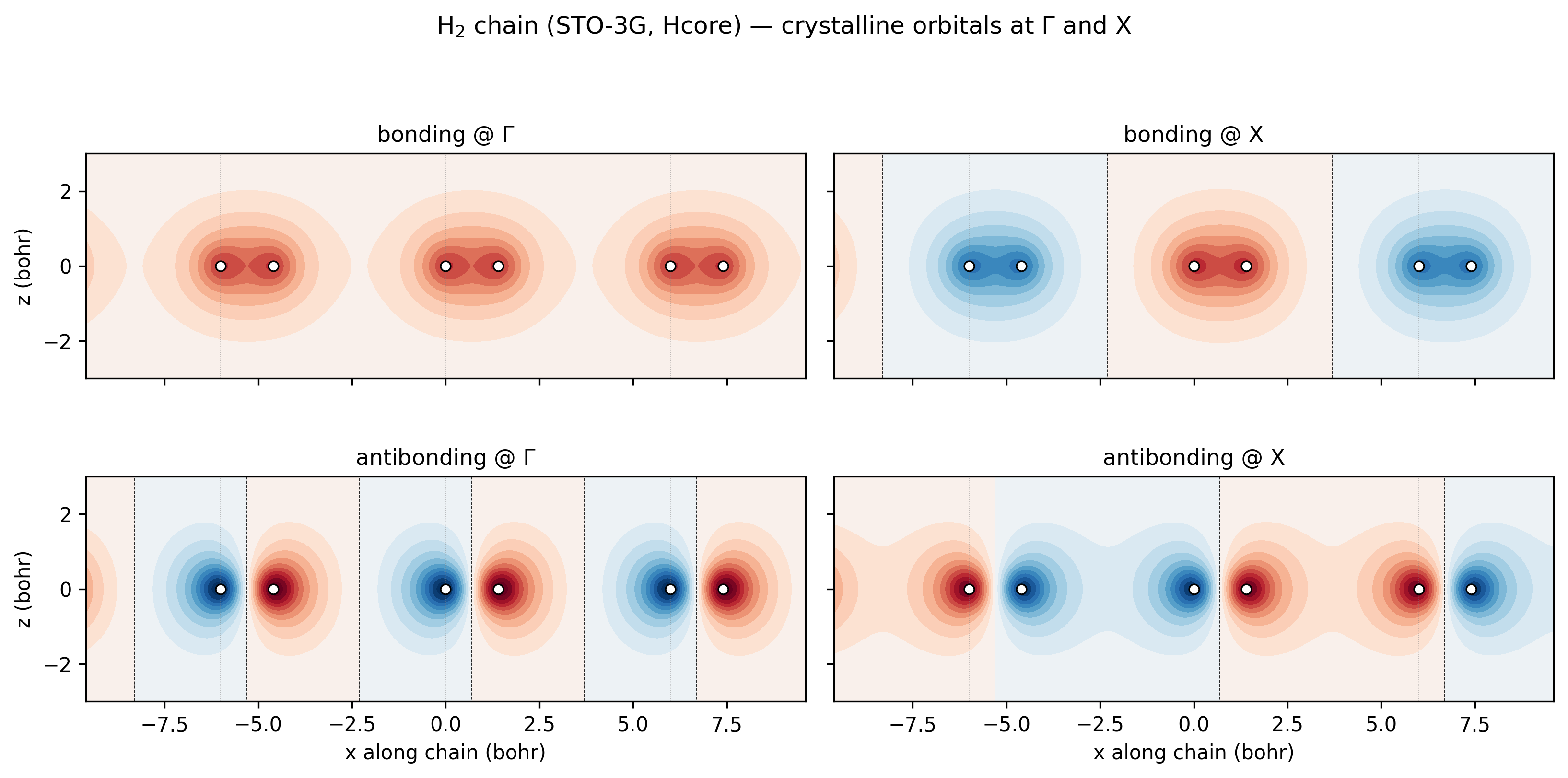
Four-panel plot of the H2-chain bonding and antibonding crystalline orbitals at Gamma and X, showing in-phase repetition at Gamma and alternating-sign repetition at X. — H₂-chain bonding and antibonding crystalline orbitals at Γ and X (STO-3G, Hcore). Three full unit cells visible; thin grey lines mark cell boundaries; white circles mark the H nuclei. **Top-left, bonding @ Γ:** every unit cell contributes its H₂ σ-bonding lobe *in phase* — the orbital is a single periodic stripe of the same sign. **Top-right, bonding @ X:** at the zone boundary the Bloch phase is \((-1)^m\) across cells, so the H₂ bonding lobes alternate sign between molecules. **Bottom-left, antibonding @ Γ:** every cell shows the same σ*-antibonding shape, with the node between the two H atoms of each molecule, all in phase. **Bottom-right, antibonding @ X:** the σ* shape alternates sign between cells.¶

Now read the bandwidths off the four panels directly: between neighbouring **bonding** lobes there’s almost no overlap (the lobes are tucked tightly between the H pairs at 1.4 bohr separation; the 4.6 bohr gaps between molecules show essentially zero amplitude), so the Γ-vs-X energy difference is tiny — the bonding band is flat. Between neighbouring **antibonding** orbitals, the outer lobes do extend into the inter-molecular region, and at X they meet opposite-sign neighbours (constructive antibonding) while at Γ they meet same-sign neighbours (destructive). That’s a real overlap difference, and it’s what gives the antibonding band its larger ~3.5 eV bandwidth.

Regenerated by `[`examples/plots/h-chain-crystalline-orbitals.py`](https://gitlab.peintinger.com/mpei/vibeqc/-/blob/main/examples/plots/h-chain-crystalline-orbitals.py)`.

The orbital plotter uses the public lattice-matrix / bloch_sum / diagonalize_bloch API to extract the MO coefficients \(C_{\mu n}(\mathbf{k})\) at each k-point, then sums

\[ \psi_{n,\mathbf{k}}(\mathbf{r}) \;=\; \sum_{\mathbf{T}} e^{i \mathbf{k} \cdot \mathbf{T}} \sum_\mu C_{\mu n}(\mathbf{k}) \, \chi_\mu(\mathbf{r} - \mathbf{T}) \]

over a window of lattice translations using evaluate_ao(basis, points - T). A first-class periodic AO evaluator (Phase V3 on the roadmap) will turn this manual recipe into a one-liner.

A multi-segment k-path¶

Real 3D Brillouin zones have many high-symmetry points. Stitch segments together:

kpath = vq.kpath_from_segments(
    system,
    [
        ((0.0, 0.0, 0.0), "Γ", (0.5, 0.0, 0.0), "X"),
        ((0.5, 0.0, 0.0), "X", (0.5, 0.5, 0.0), "M"),
        ((0.5, 0.5, 0.0), "M", (0.0, 0.0, 0.0), "Γ"),
    ],
    points_per_segment=40,
)

The plotter adds labels and ticks at each segment boundary.

Custom plotting with matplotlib¶

If you want to overlay multiple runs or style the plot for a paper, grab the raw arrays and use matplotlib directly:

import matplotlib.pyplot as plt

fig, (ax_b, ax_d) = plt.subplots(1, 2, sharey=True, figsize=(8, 4),
                                  gridspec_kw={"width_ratios": [3, 1]})

# Bands
x = bands.kpath.distances
for i in range(bands.energies.shape[1]):
    ax_b.plot(x, bands.energies[:, i] - bands.e_fermi,
              color="C0", lw=1.2)
ax_b.axhline(0.0, color="k", lw=0.5, ls="--")
# kpath.labels is [(distance, name), ...] at each high-symmetry point.
tick_pos, tick_txt = zip(*bands.kpath.labels)
ax_b.set_xticks(tick_pos)
ax_b.set_xticklabels(tick_txt)
ax_b.set_xlim(x[0], x[-1])
ax_b.set_ylabel("E - E_F (Ha)")

# DOS
ax_d.fill_betweenx(dos.energies - bands.e_fermi, dos.dos, color="C0", alpha=0.5)
ax_d.axhline(0.0, color="k", lw=0.5, ls="--")
ax_d.set_xlabel("DOS (states / Ha)")

fig.tight_layout()
fig.savefig("bands_custom.png", dpi=200)

A note on “Hcore” bands¶

band_structure_hcore / density_of_states_hcore diagonalize the kinetic + nuclear-attraction part of the Fock matrix, the non-interacting electronic structure. This is:

Fast. No SCF required, just Bloch-summed one-electron integrals and a diagonalisation at each k-point.
Correct for tight-binding-like bands. The s-only H-chain has exactly the structure you’d get from a Hückel model; Hcore nails it.
Missing electron-electron interaction. For real bands on a real solid you want HF or KS-DFT self-consistent. That path is wired through run_rhf_periodic_scf (the Coulomb-method dispatcher, see Periodic HF on a 1D H chain and the Ewald user guide) + band_structure_from_real_space. For tight-cell 2D / 3D systems, set opts.lattice_opts.coulomb_method = CoulombMethod.EWALD_3D to get unconditional Coulomb convergence.

For quick pedagogical plots Hcore is plenty.

Saving the DOS for external plotting¶

To take the DOS into another tool, dump the energy grid and the broadened density of states as two columns of a plain text file:

import numpy as np
np.savetxt("h_chain_dos.dat",
           np.column_stack([dos.energies, dos.dos]),
           header="E (Ha)    DOS (states/Ha)")

Open in gnuplot, Origin, or any plotting tool.

Periodic volumetric output¶

Crystal orbital and density visualization uses XSF / BXSF format instead of cube, see volumetric data user guide for write_xsf_volume (isosurfaces in VESTA / XCrySDen) and write_bxsf (Fermi-surface plots).

Theory¶

The sections below build up the band-structure picture from the ground: where bands come from as Bloch eigenvalues, how high-symmetry k-paths are named and sampled, how integrating over k gives the density of states, how to classify the result as metal, semimetal, or insulator, and where the non-interacting Hcore approximation departs from a self-consistent calculation.

Bands are the dispersion of Bloch eigenvalues¶

Periodic HF on a 1D H chain introduced Bloch’s theorem: every eigenstate of a translation-invariant Hamiltonian is labeled by a crystal momentum \(\mathbf{k}\) and a band index \(n\), with eigenvalue \(\varepsilon_{n}(\mathbf{k})\). A band structure plot samples \(\varepsilon_n(\mathbf{k})\) along a piecewise-linear path through the first Brillouin zone and plots each band \(n\) as a curve over the 1D path-length coordinate.

For HF / KS-DFT in a Bloch-summed AO basis, the eigenvalues come from the standard generalised eigenvalue problem at each sampled \(\mathbf{k}\):

\[ \mathbf{F}(\mathbf{k}) \, \mathbf{c}_n(\mathbf{k}) = \varepsilon_n(\mathbf{k}) \, \mathbf{S}(\mathbf{k}) \, \mathbf{c}_n(\mathbf{k}), \]

which is exactly the machinery of the periodic_hf tutorial. The non-interacting (Hcore) variant that this tutorial uses sets \(\mathbf{F} = \mathbf{h}\) (kinetic + nuclear attraction only), no electron-electron interaction, so no SCF is needed, just one diagonalisation per \(\mathbf{k}\).

High-symmetry k-paths¶

Conventional band-structure plots trace a path through named high-symmetry points of the BZ, Γ, X, M, L, K, …, where the stars denote points whose site group in the BZ has extra symmetry and where the bands often touch or cross. The naming follows Setyawan-Curtarolo 2010 for most lattice types. A typical path for a simple cubic BZ is Γ → X → M → Γ → R → X; vibe-qc’s kpath_from_segments takes arbitrary segments and produces a dense sampling with arc-length parametrisation.

Density of states¶

Integrating out the crystal momentum gives the density of states:

\[ \mathrm{DOS}(E) = \sum_n \int_\text{BZ} \delta\bigl(E - \varepsilon_n(\mathbf{k})\bigr) \, \frac{\mathrm{d}^3 k}{(2\pi)^3}. \]

Practical implementations replace the \(\delta\) function with a narrow Gaussian of width \(\sigma\) (or a Methfessel-Paxton smearing function) evaluated on a uniform k-mesh. vibe-qc’s default is \(\sigma = 0.02\) Ha \(\approx 0.54\) eV. At the Fermi level, \(\mathrm{DOS}(E_F) = 0\) for an insulator and \(> 0\) for a metal, the single most-useful diagnostic the DOS provides.

Gap, metal, semimetal¶

Classifying a band structure:

Feature	Name
Valence band maximum below conduction band minimum; \(\mathrm{DOS}(E_F) = 0\)	Insulator (semiconductor if gap \(\lesssim 3\) eV)
VBM and CBM at the same \(\mathbf{k}\)	Direct gap
VBM and CBM at different \(\mathbf{k}\)	Indirect gap
Bands cross \(E_F\)	Metal
Bands touch but don’t cross (linear dispersion around touching)	Semimetal (graphene, some Dirac/Weyl semimetals)

The single-point H₂-chain example above has a clean direct gap at both Γ and X, widely separated, no metallic character.

Non-interacting vs. self-consistent bands¶

This tutorial’s band_structure_hcore diagonalises only the kinetic-plus-nuclear part of the Fock matrix, a tight-binding-like model with no electron-electron interaction. For a real solid you want the self-consistent bands from an HF or KS-DFT SCF at the chosen k-mesh, then Fourier-transform the converged real-space Fock matrix to your chosen k-path and diagonalize. That path is wired through band_structure (drop the _hcore) once you have a LatticeMatrixSet from a converged SCF. Quantitative 3D band structures still wait for the tight-cell SCF convergence tooling the roadmap tracks.

Resources¶

~150 MB peak RAM, ~1 s on one core (Apple M2 baseline) for the H₂-chain Hcore bands + DOS example. Hcore is the cheapest way to plot bands, it skips the SCF iteration entirely. A full periodic SCF adds the wall time of the underlying run_rhf_periodic_scf call (see Periodic HF on a 1D H chain).

References¶

Bloch’s theorem. F. Bloch, “Über die Quantenmechanik der Elektronen in Kristallgittern,” Z. Phys. 52, 555 (1929).
High-symmetry k-paths. W. Setyawan and S. Curtarolo, “High-throughput electronic band structure calculations: challenges and tools,” Comput. Mater. Sci. 49, 299 (2010).
DOS smearing. M. Methfessel and A. T. Paxton, “High-precision sampling for Brillouin-zone integration in metals,” Phys. Rev. B 40, 3616 (1989).
Textbook, band structure. N. W. Ashcroft and N. D. Mermin, Solid State Physics, Cengage Learning reprint (1976), chapters 8-9.
Modern review, solid-state electronic structure. R. M. Martin, Electronic Structure: Basic Theory and Practical Methods, 2nd ed., Cambridge University Press (2020). Chapter 10 covers Bloch representation; chapter 14 covers k-space integration.

Next¶

This is the first solid-state tutorial built on the matured periodic infrastructure; more will follow (full-SCF bands, phonons, surface cells) as the periodic SCF convergence tooling lands.