Nudged elastic band: reaction paths and transition states

Geometry optimization (the geometry_optimization tutorial) finds minima. Transition-state search finds first-order saddle points, the structures where a reaction actually happens. The Nudged Elastic Band (NEB) algorithm does this by threading a chain of intermediate geometries (“images”) between two minima, connecting them with fictitious springs, and relaxing the chain onto the minimum-energy path on the PES. The highest-energy image approximates the transition state.

This tutorial walks through the canonical closed-shell example: NH₃ umbrella inversion, the molecule flips through a planar (D₃h) transition state to invert its chirality.

The one-liner

vibe-qc finds reaction paths natively with run_neb, pass the two endpoints, a basis, and climbing_image=True:

import vibeqc as vq

result = vq.run_neb(reactant, product, basis="sto-3g", method="RHF",
                    n_images=5, climbing_image=True)
ts = result.path.images[result.transition_state_index].system

run_neb builds the interpolated band, runs the per-image SCFs (in parallel if you ask), assembles the improved-tangent NEB force, and relaxes the band with a quick-min outer loop, vibe-qc’s own code end to end. The full worked example lives in examples/workflows/input-nh3-umbrella-neb.py; this page walks through its key pieces. Prefer to drive NEB from an ASE workflow? See Driving NEB through ASE at the end.

Build the two endpoints

Two copies of pyramidal NH₃, one with H atoms below the nitrogen, one above, each relaxed to its minimum with vibe-qc’s optimiser. vibe-qc coordinates are in bohr, so the experimental geometry (quoted in Å) is converted on the way in:

import numpy as np
import vibeqc as vq

ANG_TO_BOHR = 1.8897259886

def build_nh3(flip=False):
    theta = np.deg2rad(106.67)          # experimental HNH angle
    r_nh = 1.012 * ANG_TO_BOHR          # experimental N-H (1.012 Å → bohr)
    sin_a = np.sqrt(2 * (1 - np.cos(theta)) / 3)
    cos_a = np.sqrt(1 - sin_a**2)
    z_sign = +1 if flip else -1
    atoms = [vq.Atom(7, [0.0, 0.0, 0.0])]       # nitrogen at origin
    for k in range(3):
        phi = k * 2 * np.pi / 3
        atoms.append(vq.Atom(1, [
            r_nh * sin_a * np.cos(phi),
            r_nh * sin_a * np.sin(phi),
            z_sign * r_nh * cos_a,
        ]))
    return vq.Molecule(atoms, 0, 1)             # neutral singlet

reactant = vq.optimize_molecule(build_nh3(flip=False), "sto-3g", method="rhf").system
product  = vq.optimize_molecule(build_nh3(flip=True),  "sto-3g", method="rhf").system

Both relax to equivalent pyramidal minima related by mirror symmetry

• same energy, mirror-image geometry. optimize_molecule returns a result object; its .system is the relaxed Molecule.

Run the climbing-image band

With both minima in hand, a single run_neb call threads the band between them and relaxes it. The three options that matter for this inversion are spelled out right after the call:

result = vq.run_neb(
    reactant, product,
    basis="sto-3g",
    n_images=5,                          # 5 interior images + 2 endpoints
    method="RHF",
    interpolation="linear",              # smooth flip, no bonds break → IDPP not needed
    climbing_image=True,
    climbing_image_start_fraction=0.1,   # promote the climber early (see note)
    conv_tol_force=1e-3,                 # ≈ 0.05 eV/Å, the Kolsbjerg 2016 default
)

Three choices matter here:

1. climbing_image=True. Without climbing, the image near the peak is pulled down by its neighbouring springs and never sits at the TS. With climbing on, the highest-energy image is freed from the spring force and pushed uphill along the tangent, it converges onto the exact saddle point.

2. climbing_image_start_fraction=0.1. The climber is promoted only after a plain-NEB warm-up (default 0.3 × max_iter) so the band settles before one image starts climbing. This small, symmetric band converges in ~56 iterations, faster than the default warm-up would engage, so we shorten the warm-up to let the climber take over in time. On larger barriers the default is usually fine.

3. interpolation="linear". The umbrella flip is a smooth geometric motion with no change in bonding, so a straight-line interpolation seeds the band well. For reactions that break or form bonds, use "idpp" (image-dependent pair potential), which avoids atom-atom clashes in the starting path.

There is no optimizer to choose: run_neb uses a quick-min (damped-MD) outer loop internally, which is the right integrator for the non-conservative NEB force (see Theory). On this system the band converges in well under two seconds on a single core; pass n_jobs=-1 to parallelise the per-image SCFs across cores for bigger problems.

Read the MEP

The converged band carries one energy per image. Referencing each to the first endpoint and converting to kcal/mol traces the minimum-energy path and exposes the barrier height:

e = result.energies                      # per-image energies (Hartree)
for i, de in enumerate((e - e[0]) * 627.509):
    print(f"image {i}: ΔE = {de:+.3f} kcal/mol")

Output:

image 0: ΔE = +0.000 kcal/mol
image 1: ΔE = +0.002 kcal/mol
image 2: ΔE = +1.675 kcal/mol
image 3: ΔE = +11.141 kcal/mol    ← TS
image 4: ΔE = +1.675 kcal/mol
image 5: ΔE = +0.002 kcal/mol
image 6: ΔE = -0.000 kcal/mol

Symmetric about image 3, as expected for the symmetric inversion. result.transition_state_index is 3 (the highest-energy image, which is also result.path.climbing_image_index once the climber is promoted); image 3 is the transition state, at 11.1 kcal/mol above the pyramidal minimum.

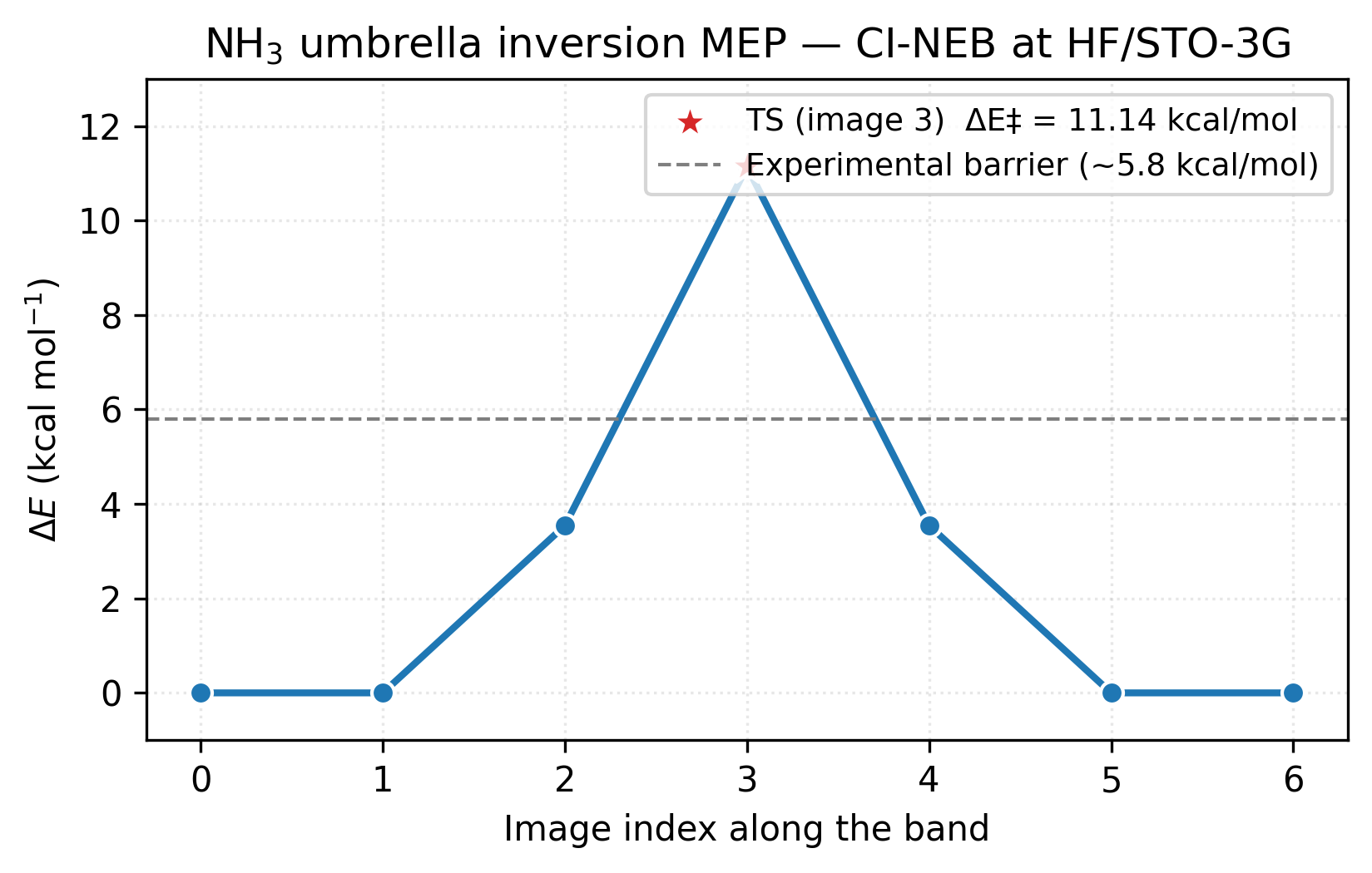
The figure makes the symmetry visible at a glance: the path is its own mirror image around the climbing image (red star) at index 3. Images 1 and 5 sit essentially flat against the endpoint minima, the band only starts climbing at images 2 and 4 as the molecule flattens. The dashed grey line marks the experimental barrier (~5.8 kcal/mol); HF/STO-3G overshoots by nearly 2× because the sp³→sp² rehybridisation at the TS is exactly the regime where electron correlation stabilises the more delocalised state and a minimum basis cannot describe it. The shape of the path is right at every level of theory; the height needs MP2 or hybrid DFT in a TZ-quality basis to match experiment.

The plot is regenerated by [examples/plots/nh3-umbrella-neb-mep.py](https://gitlab.peintinger.com/mpei/vibeqc/-/blob/main/examples/plots/nh3-umbrella-neb-mep.py) from the trajectory written by the example script.

Inspect the TS

Pulling the highest-energy image out of the band and printing its atom positions (converted back to Å) confirms the saddle point is the planar D₃h structure the two pyramidal minima invert through:

BOHR_TO_ANG = 0.52917721067
ts = result.path.images[result.transition_state_index].system
for a in ts.atoms:
    x, y, z = np.array(list(a.xyz)) * BOHR_TO_ANG
    print(f"  {('N' if a.Z == 7 else 'H')}   {x:+.3f}  {y:+.3f}  {z:+.3f}")

  N   +0.000  +0.000  +0.000
  H   +1.005  +0.000  +0.000    ← all H at z=0
  H   -0.503  +0.871  +0.000
  H   -0.503  -0.871  +0.000

All three H atoms sit at \(z = 0\), the planar D₃h transition state that connects the two pyramidal enantiomers. N-H bond length (1.005 Å) is a touch shorter than the pyramidal equilibrium (1.012 Å): the in-plane geometry is sp²-like and the overlap tightens.

Comparing to experiment

The computed barrier depends strongly on the level of theory. The table below tracks the NH₃ inversion barrier from HF/STO-3G up to MP2/aug-cc-pVTZ against the experimental value:

Level	NH₃ barrier (kcal/mol)
HF/STO-3G	11.14
HF/6-31G**	~6.0
MP2/aug-cc-pVTZ	~5.7
Experimental	~5.8

HF/STO-3G over-estimates by nearly 2×, a reminder that tutorial numbers are qualitative until you climb the basis and correlation hierarchies. The shape of the path (symmetric, planar TS, one barrier) is qualitatively right at every level.

Animate the path

The example script writes two renderable artefacts of the converged band: a vibe-view archive via result.write_qvf(...) (output-nh3-umbrella-neb.qvf, drop it into vibe-view for an interactive reaction-path animation with the per-image energy plot), and output-nh3-umbrella-neb.traj, an ASE trajectory of all seven images. The path animates as a ping-pong loop forward through the inversion and back:

The 3D molecule on the left flips through the seven NEB images while the right inset highlights which image is currently shown on the MEP curve. Reactant (image 1) and product (image 7) are mirror images of each other through the planar TS at image 4, the classic D₃ₕ transition state of the umbrella inversion.

For interactive inspection (rotation, atom labeling, distance measurement), open the trajectory in ASE’s GUI:

ase gui output-nh3-umbrella-neb.traj

Space advances one frame. Reproduce the GIF above with python3 examples/plots/nh3-umbrella-neb-animation.py.

Driving NEB through ASE

run_neb is the native path and the one this tutorial recommends. But vibe-qc also exposes an ASE Calculator, so you can drive NEB (and the dimer method, IRC, …) through ASE’s own optimizers when you are already in an ASE workflow:

from ase import Atoms
from ase.mep import NEB
from ase.optimize import FIRE
from vibeqc.ase import VibeQC

# initial / final: relaxed ASE Atoms, each with atoms.calc = VibeQC(basis="sto-3g")
images = [initial] + [initial.copy() for _ in range(5)] + [final]
for img in images:
    img.calc = VibeQC(basis="sto-3g")           # every image needs its own calc

neb = NEB(images, k=0.1, climb=True, method="improvedtangent")
neb.interpolate()
FIRE(neb, logfile=None).run(fmax=0.05, steps=200)   # FIRE, not BFGS — see Theory

This converges to the same TS barrier (11.14 kcal/mol). The ASE route is also how you reach ASE’s own dimer-method and IRC drivers, though vibe-qc implements both natively as well (run_dimer, run_irc); see What NEB doesn’t find.

Theory

The sections below unpack how NEB works: the spring-coupled band construction and the forces on each image, why the per-step cost is far smaller than the image count suggests, the climbing-image trick that pins the top image onto the saddle, and the related searches NEB cannot perform.

The NEB construction

Given initial and final geometries \(\mathbf{R}_0\) and \(\mathbf{R}_N\), NEB inserts \(N-1\) intermediate images \(\mathbf{R}_1, \dots, \mathbf{R}_{N-1}\) and connects consecutive images with fictitious springs. Each intermediate image feels two forces:

1. Perpendicular PES force, the true gradient of the electronic energy projected onto the direction perpendicular to the band tangent \(\hat{\tau}_i\):

   \[ \mathbf{F}_i^\perp = -\nabla E(\mathbf{R}_i) + (\nabla E(\mathbf{R}_i) \cdot \hat{\tau}_i)\, \hat{\tau}_i. \]

2. Parallel spring force, along the tangent, with spring constant \(k\), keeps the images from collapsing into the endpoints:

   \[ \mathbf{F}_i^\parallel = k \bigl( |\mathbf{R}_{i+1} - \mathbf{R}_i| - |\mathbf{R}_i - \mathbf{R}_{i-1}| \bigr) \hat{\tau}_i. \]

The total NEB force \(\mathbf{F}_i^\text{NEB} = \mathbf{F}_i^\perp + \mathbf{F}_i^\parallel\) is not the gradient of any scalar, the spring term depends only on the parallel projection of the displacement, so no scalar potential has it as a gradient. This is why a standard BFGS line-search (which assumes an energy it can decrease) fails on NEB, and why run_neb uses a quick-min (damped-MD) outer loop instead. At convergence (\(\mathbf{F}_i^\text{NEB} = \mathbf{0}\) for every interior \(i\)), the band traces the minimum-energy path on the PES. The improved-tangent variant (Henkelman-Jónsson 2000), run_neb’s default, uses a smarter tangent definition that avoids kinking on asymmetric paths.

Why NEB is so much cheaper than it looks

Each NEB optimization step evaluates the gradient on every intermediate image, seemingly \(N\)× the cost of a single gradient. But in practice (a) the images at each step are close enough that SCF converges in a handful of iterations each, and run_neb reuses each image’s converged density across outer iterations (warm_start=True, the default) so the SCF starts warm rather than from scratch; and (b) the per-image SCFs at each step are independent, so n_jobs=-1 spreads them across cores. For a 5-image band on a small molecule, you’re looking at \(\mathcal{O}(100)\) single-point SCFs, comparable to a single geometry optimization.

The climbing-image trick

Plain NEB leaves the highest-energy image pulled slightly below the true saddle point by the spring force from its neighbors. The climbing image variant (Henkelman, Uberuaga, Jónsson 2000) identifies the highest-energy image and replaces its force with

\[ \mathbf{F}_\text{ci}^\text{CI-NEB} = -\nabla E(\mathbf{R}_\text{ci}) + 2\,(\nabla E(\mathbf{R}_\text{ci}) \cdot \hat{\tau})\, \hat{\tau}, \]

• the true PES gradient with the tangent component inverted. This drives the climbing image uphill along the tangent (toward the TS) and downhill perpendicular (onto the ridge). The result is that the climbing image converges to the exact saddle point, not just close to it. Cost-wise: negligible extra work. (On a perfectly symmetric path like this one, plain NEB already lands the centre image on the saddle by symmetry; climbing matters most on asymmetric barriers.)

What NEB doesn’t find

NEB only walks a path between two pre-specified minima. If the mechanism you’re looking for goes via an intermediate you didn’t anticipate, NEB gives you a suboptimal path with multiple local maxima. Complements:

• Intrinsic Reaction Coordinate (IRC), starts from an already-known TS and traces the path downhill in both directions to identify the connected minima. This ships natively as vq.run_irc, the natural follow-up to a dimer/NEB saddle search:

  irc = vq.run_irc(ts, basis="sto-3g", method="RHF")   # auto imaginary mode
  reactant, product = irc.reverse_minimum, irc.forward_minimum
  

• Dimer method / eigenvector-following, finds saddle points from a single starting geometry plus a direction, no pre-specified endpoints needed. This ships natively as vq.run_dimer (same SCF / MACE method surface as run_neb):

  result = vq.run_dimer(start, basis="sto-3g", method="RHF",
                        initial_direction=mode)   # guessed reaction direction
  ts = result.system                              # result.is_saddle, result.curvature
  

• Metadynamics / enhanced sampling, explores the PES adaptively, good for systems where the mechanism is genuinely unknown.

Metadynamics doesn’t ship natively yet; ASE has a module for it that drives through the VibeQC calculator exactly like the ASE NEB route above.

Resources

~150 MB peak RAM, ~1.5 s on one core (Apple M2 baseline) for the seven-image NH₃ NEB at HF/STO-3G: 5 interior images × ~56 quick-min iterations × (HF + analytic gradient), run serially. Cost scales linearly in (image count × NEB step count × per-image SCF cost), bigger barriers and slower-converging bands quickly push the wall time into hours, at which point n_jobs=-1 (parallelising the per-image SCFs across cores) becomes worth it.

References

• Original NEB formulation. H. Jónsson, G. Mills, and K. W. Jacobsen, “Nudged elastic band method for finding minimum energy paths of transitions,” in Classical and Quantum Dynamics in Condensed Phase Simulations, B. J. Berne, G. Ciccotti, and D. F. Coker eds., World Scientific (1998), p. 385.

• Improved tangent variant. G. Henkelman and H. Jónsson, “Improved tangent estimate in the nudged elastic band method for finding minimum energy paths and saddle points,” J. Chem. Phys. 113, 9978 (2000).

• Climbing-image NEB. G. Henkelman, B. P. Uberuaga, and H. Jónsson, “A climbing image nudged elastic band method for finding saddle points and minimum energy paths,” J. Chem. Phys. 113, 9901 (2000).

• FIRE optimizer. E. Bitzek, P. Koskinen, F. Gähler, M. Moseler, and P. Gumbsch, “Structural relaxation made simple,” Phys. Rev. Lett. 97, 170201 (2006).

• ASE NEB implementation. A. H. Larsen et al., “The atomic simulation environment, a Python library for working with atoms,” J. Phys. Condens. Matter 29, 273002 (2017). Section 3.4.

• Ammonia inversion barrier, experimental. J. D. Swalen and J. A. Ibers, “Potential function for the inversion of ammonia,” J. Chem. Phys. 36, 1914 (1962).

Next

• Once you have a TS, vibrational frequencies on it should show exactly one imaginary mode aligned with the reaction coordinate

  • see Vibrational frequencies. ASE’s Vibrations on an NEB TS image makes this a two-line check.

• Thermodynamics gives ΔG‡ = barrier + zero-point + entropy corrections, bringing you from an electronic barrier to an Eyring-equation rate constant.

• For bigger mechanisms (reactive systems with more than two minima), stitch NEB runs together via shared images.