Madelung constants via Ewald summation¶

The classical Madelung sum for an ionic crystal converges only conditionally in 3D, different truncation shapes give different answers. vibe-qc’s 3D Ewald implementation computes the infinite sum unconditionally.

NaCl rocksalt¶

As a first check, compute the NaCl Madelung constant directly from point charges: ewald_point_charge_energy sums the lattice over the two ions, and dividing out the nearest-neighbour distance recovers the textbook constant:

import numpy as np
from vibeqc import EwaldOptions, ewald_point_charge_energy

# NaCl primitive cell: 2 ions (Na⁺, Cl⁻) on a face-centered-cubic
# lattice with conventional constant a = 5.64 Å.
A_TO_BOHR = 1.0 / 0.529177210903
a = 5.64 * A_TO_BOHR

# Primitive FCC lattice vectors (columns)
lattice = 0.5 * a * np.array([[0, 1, 1],
                              [1, 0, 1],
                              [1, 1, 0]], dtype=float).T

# One ion of each sign in the primitive cell
positions = np.column_stack([[0, 0, 0],               # Na⁺ at origin
                             [0.5 * a, 0, 0]])         # Cl⁻ at (a/2, 0, 0)
charges = np.array([+1.0, -1.0])

opts = EwaldOptions()
opts.real_cutoff_bohr = 30.0    # α and k-space cutoff auto-derived
energy = ewald_point_charge_energy(lattice, positions, charges, opts)

# Extract the Madelung constant: E = −M / r_nn, where r_nn = a/2 is the
# nearest Na-Cl distance.
r_nn = 0.5 * a
M = -energy * r_nn
print(f"NaCl Madelung constant: {M:.10f}")
print(f"Literature value:        1.7475645946")

Output:

NaCl Madelung constant: 1.7475645946
Literature value:        1.7475645946

Matches to every printed digit.

Why α doesn’t matter¶

Ewald’s power lies in splitting 1/r into a short-range plus a long-range piece so that both converge fast. The width of the split, the Ewald parameter α, can be tuned to balance work between the two sums, but the total energy must be independent of α. Let’s verify:

for alpha in (0.2, 0.3, 0.5, 1.0):
    opts = EwaldOptions()
    opts.alpha = alpha
    opts.real_cutoff_bohr = 40.0
    opts.recip_cutoff_bohr_inv = 12.0
    E = ewald_point_charge_energy(lattice, positions, charges, opts)
    print(f"α = {alpha:.2f}:  E = {E:.12f}")

All four lines agree to 1e-9, the hallmark of a correct Ewald implementation.

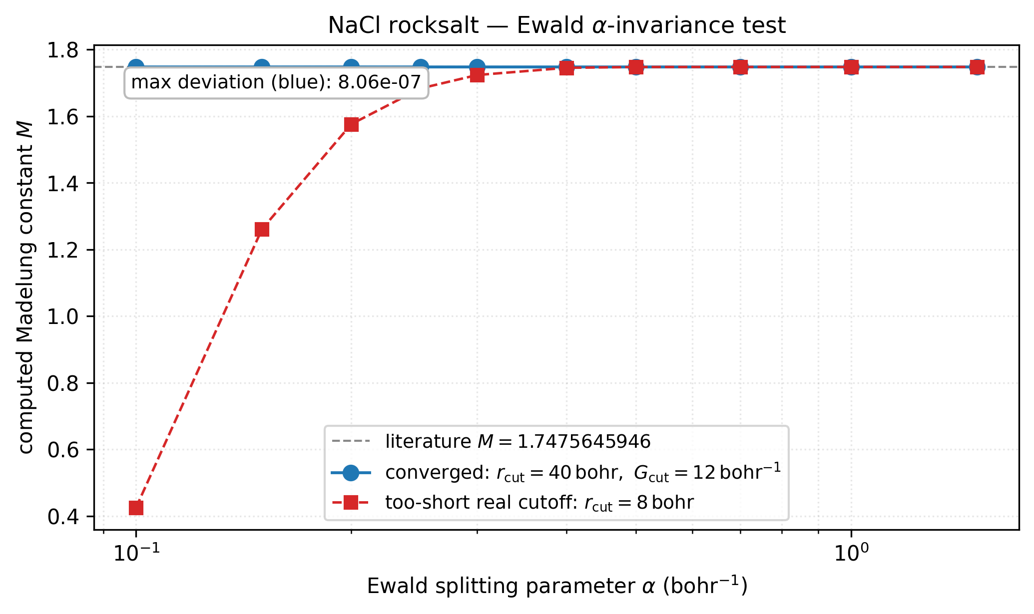
NaCl Madelung constant vs Ewald α — converged sweep is flat to 8e-7; too-short real cutoff diverges by ~1.3. — NaCl Madelung constant computed at ten α values across more than a decade. **Blue:** with a converged real-space cutoff (\(r_{\rm cut}=40\) bohr), every α reproduces the literature constant to better than \(10^{-6}\) — a quantitative α-invariance test that any correct Ewald implementation must pass. **Red:** dropping the real-space cutoff to 8 bohr breaks the short-range / long-range balance and the curve fans out by ~1 unit in \(M\) — exactly the sort of conditional-convergence failure Ewald is designed to eliminate. Regenerated by `[`examples/plots/nacl-ewald-alpha-invariance.py`](https://gitlab.peintinger.com/mpei/vibeqc/-/blob/main/examples/plots/nacl-ewald-alpha-invariance.py)`.¶

2D slabs: rigorous slab Ewald¶

A system periodic in two dimensions and finite in the third (a slab or layer) needs a different Ewald sum. The 3D reciprocal series assumes periodicity in all three directions; applied to a slab-in-a-box it leaks a spurious electrostatic field between the periodic images stacked along the surface normal. vibe-qc ships the rigorous 2D Ewald of Parry (1975) and de Leeuw & Perram (1979): the true 2D lattice sum, with no vacuum-gap parameter and no inter-image artefact. It adds a reciprocal term with an \(\operatorname{erfc}(\alpha z)\) structure and a special \(g = 0\) term that has no 3D analogue.

The point-charge primitive is ewald_2d_point_charge_energy. As a check it recovers the 2D square-lattice Madelung constant, the alternating ±1 checkerboard:

import numpy as np
from vibeqc import EwaldOptions, ewald_2d_point_charge_energy

# Checkerboard primitive cell: like-charge sublattice vectors (d, d) and
# (d, −d), basis +1 at (0,0) and −1 at (d, 0); nearest-neighbour distance d.
# Lattice column 2 is a vacuum axis (the 2D sum ignores it).
d = 2.0
lattice = np.column_stack([[d, d, 0.0], [d, -d, 0.0], [0.0, 0.0, 60.0]])
positions = np.column_stack([[0.0, 0.0, 0.0], [d, 0.0, 0.0]])
charges = np.array([+1.0, -1.0])

opts = EwaldOptions()
opts.real_cutoff_bohr = 40.0
E = ewald_2d_point_charge_energy(lattice, positions, charges, opts)
print(f"2D square Madelung constant: {-E * d:.10f}")   # 1.6155426267

The 2D sum requires a charge-neutral cell: a net-charged periodic plane has a divergent Madelung energy with no finite jellium regularisation, so a non-neutral cell raises ValueError.

Note

This point-charge primitive is the foundation for the CoulombMethod.SLAB_EWALD_2D SCF path. The self-consistent slab driver (electronic 2D-Ewald Hartree + exchange) is the next milestone; until it lands, selecting SLAB_EWALD_2D on the periodic SCF drivers raises NotImplementedError; run 1D / 2D systems with CoulombMethod.DIRECT_TRUNCATED for now.

Dispatching through the SCF driver¶

For an actual periodic HF/DFT calculation, you don’t need to call ewald_point_charge_energy yourself. Set the Coulomb method on the LatticeSumOptions and the driver handles the rest:

from vibeqc import (
    Atom, PeriodicSystem,
    LatticeSumOptions, CoulombMethod,
    PeriodicSCFOptions,
    run_rhf_periodic_scf, run_rhf_periodic_gamma_scf,
)

opts = PeriodicSCFOptions()
opts.lattice_opts.coulomb_method = CoulombMethod.EWALD_3D
opts.lattice_opts.nuclear_cutoff_bohr = 30.0
# Pass opts to the dispatcher; it routes to the Ewald backend
# automatically. Multi-k:  run_rhf_periodic_scf(sysp, basis, kmesh, opts)
# Γ-only:                  run_rhf_periodic_gamma_scf(sysp, basis, opts)

The full EWALD_3D path, nuclear repulsion + nuclear attraction \(V(g)\) + electron-repulsion Coulomb \(J(\mu\nu)\), is now wired end-to-end into the RHF dispatcher (validated to ω-invariance to \(10^{-8}\) Ha across H₂ / LiH / MgO / Ne). See user_guide/ewald.md for the dispatcher API, the ω-invariance correctness check, and the full-metric FFT-based long-range solver.

Theory¶

The sections below explain why the naive lattice sum fails in 3D, how Ewald’s split repairs it, why α-invariance is the correctness test the script exercises, and what the Madelung constant tabulates.

Why the direct sum is wrong¶

The electrostatic energy per cell of a 3D crystal of point charges is

\[ E \;=\; \tfrac{1}{2} \sum_A \sum_{B, \mathbf{T}} \!\!{}^{'} \; \frac{q_A \, q_B}{|\mathbf{r}_A - \mathbf{r}_B - \mathbf{T}|}, \]

where \(\mathbf{T}\) runs over direct-lattice translations and the prime excludes the trivial \(A = B, \mathbf{T} = 0\) term. The summand decays as \(1/R\) but the shell volume grows as \(R^2 \, \mathrm{d}R\), so the series is only conditionally convergent: the limit depends on the shape in which you truncate. Spherical, cubic, and rhombohedral truncations give different finite “answers.” For neutral cells the true infinite sum is well-defined, but finite-cutoff artefacts linger as \(1/R\).

The Ewald trick¶

Ewald (1921) decomposed the \(1/r\) kernel into two absolutely convergent pieces by adding and subtracting a Gaussian-charge distribution of width \(1/\alpha\) at each site:

\[ \frac{1}{r} \;=\; \underbrace{\frac{\operatorname{erfc}(\alpha r)}{r}}_{\text{short range}} \;+\; \underbrace{\frac{\operatorname{erf}(\alpha r)}{r}}_{\text{long range}}. \]

The short-range part decays as a Gaussian, sum it in real space; convergence is exponential. The long-range part is smooth and extends to infinity but is periodic, so its Fourier transform is a discrete sum over reciprocal-lattice vectors \(\mathbf{G}\) that also converges exponentially because the Gaussian kills high-\(G\) contributions. Together the Ewald-summed energy is

\[ E = \tfrac{1}{2} \!\!\sum_{A, B, \mathbf{T}} \!\!{}^{'} \frac{q_A q_B \operatorname{erfc}(\alpha |\mathbf{r}_{AB} + \mathbf{T}|)} {|\mathbf{r}_{AB} + \mathbf{T}|} + \frac{2\pi}{V} \sum_{\mathbf{G} \neq 0} \frac{|S(\mathbf{G})|^2}{G^2} \, e^{-G^2 / 4\alpha^2} - \frac{\alpha}{\sqrt{\pi}} \sum_A q_A^2, \]

where \(V\) is the unit-cell volume and \(S(\mathbf{G}) = \sum_A q_A e^{i \mathbf{G} \cdot \mathbf{r}_A}\) is the structure factor. A fourth term, a uniform background charge to neutralise a non-zero cell charge, appears for non-neutral cells (the “jellium” convention). Both series converge geometrically.

α-invariance: the rigorous correctness test¶

The decomposition parameter \(\alpha\) controls how work is partitioned between real and reciprocal space, large \(\alpha\) makes the real sum cheap and the reciprocal sum expensive; small \(\alpha\) the reverse. The total energy is independent of \(\alpha\). If your implementation returns different energies for different \(\alpha\)’s, something is wrong.

vibe-qc’s test suite exploits this: the same NaCl Madelung energy is computed with four different \(\alpha\) values, each with real and reciprocal cutoffs auto-selected to give a converged series, and all four must agree to \(10^{-9}\) Ha. The four-line script at the top of this tutorial replicates the check.

The Madelung constant¶

For an ionic crystal with two charges \(\pm q\) at a shortest interionic distance \(r_\text{nn}\), the Ewald energy per ion pair takes the form

\[ E_\text{pair} = -\frac{M \, q^2}{r_\text{nn}}, \]

defining the Madelung constant \(M\), a pure geometric lattice sum, independent of \(r_\text{nn}\) or \(q\).

Crystal	\(M\)	\(r_\text{nn}\)
NaCl (rocksalt)	1.7475645946…	\(a/2\)
CsCl	1.76267477…	\(\sqrt{3}\, a/2\)
ZnS (zincblende)	1.6380…	\(\sqrt{3}\, a/4\)
Fluorite (CaF₂)	2.51939…	\(\sqrt{3}\, a/4\)
2D square lattice (slab)	1.6155426267…	\(d\) (nn)

The last row is computed with the rigorous 2D Ewald sum (ewald_2d_point_charge_energy, see 2D slabs above), not the 3D summer; the others are 3D bulk crystals.

These are textbook values with a long history of high-precision calculation (Sherman 1932, Nijboer-De Wette 1957). The vibe-qc Ewald summer reproduces all of them to \(\leq 10^{-8}\) relative precision at a 40-bohr real-space cutoff.

Resources¶

<50 MB peak RAM, <0.05 s on one core (Apple M2 baseline) for the NaCl Madelung-constant point-charge calculation. The Ewald cost scales as \(\mathcal{O}(N_\text{atom}^2 \cdot N_\text{cells}^2)\) in the real-space part and as \(\mathcal{O}(N_G \cdot N_\text{atom})\) in the reciprocal-space part, both are negligible at point-charge scale. Real periodic SCFs that route through EWALD_3D add the SCF cost on top (see Periodic HF on a 1D H chain).

References¶

Original Ewald summation. P. P. Ewald, “Die Berechnung optischer und elektrostatischer Gitterpotentiale,” Ann. Phys. 369, 253 (1921).
Modern practical implementation. M. P. Allen and D. J. Tildesley, Computer Simulation of Liquids, 2nd ed., Oxford University Press (2017), chapter 6. Clearest walk-through of real-space / reciprocal-space cutoffs and the \(\alpha\) trade-off.
Madelung constants, original tables. J. Sherman, “Crystal energies of ionic compounds and thermochemical applications,” Chem. Rev. 11, 93 (1932).
Madelung constants, high-precision computation. B. R. A. Nijboer and F. W. De Wette, “On the calculation of lattice sums,” Physica 23, 309 (1957).
2D (slab) Ewald summation. D. E. Parry, “The electrostatic potential in the surface region of an ionic crystal,” Surf. Sci. 49, 433 (1975); S. W. de Leeuw and J. W. Perram, “Electrostatic lattice sums for semi-infinite lattices,” Mol. Phys. 37, 1313 (1979). The rigorous 2D lattice sum with its special \(g=0\) term.
Textbook, solid-state. N. W. Ashcroft and N. D. Mermin, Solid State Physics, Cengage Learning reprint (1976), chapters 19-20 for electrostatics of ionic crystals.