Working with vibe-view¶

You will learn: how to produce a .qvf archive from vibe-qc, open it in vibe-view, inspect every section the calculation wrote, and use the headless capture API to generate publication-quality figures from scripts or CI pipelines. We cover molecular (H2O) and periodic (Si diamond) workflows and walk through all 38 section kinds the viewer renders, plus import/export formats, bond analysis, compare mode, and QA validation.

Prerequisites:

vibeqc installed and a working SCF setup.
vibe-view installed: from the vibe-qc checkout root, pip install -e vibe-view/.
A modern browser.

Time to complete: about 30 minutes.

Minimum example¶

# input-h2o.py
from vibeqc import Atom, Molecule, run_job

mol = Molecule([
    Atom(8, [0.0,  0.00,  0.00]),
    Atom(1, [0.0,  1.43, -0.98]),
    Atom(1, [0.0, -1.43, -0.98]),
])

run_job(
    mol,
    basis="6-31g*",
    method="rks",
    functional="PBE",
    output="h2o",
    output_qvf=True,
    write_cube=["density", "homo", "lumo"],
    write_molden_file=True,
    hessian=True,
    optimize=True,
)

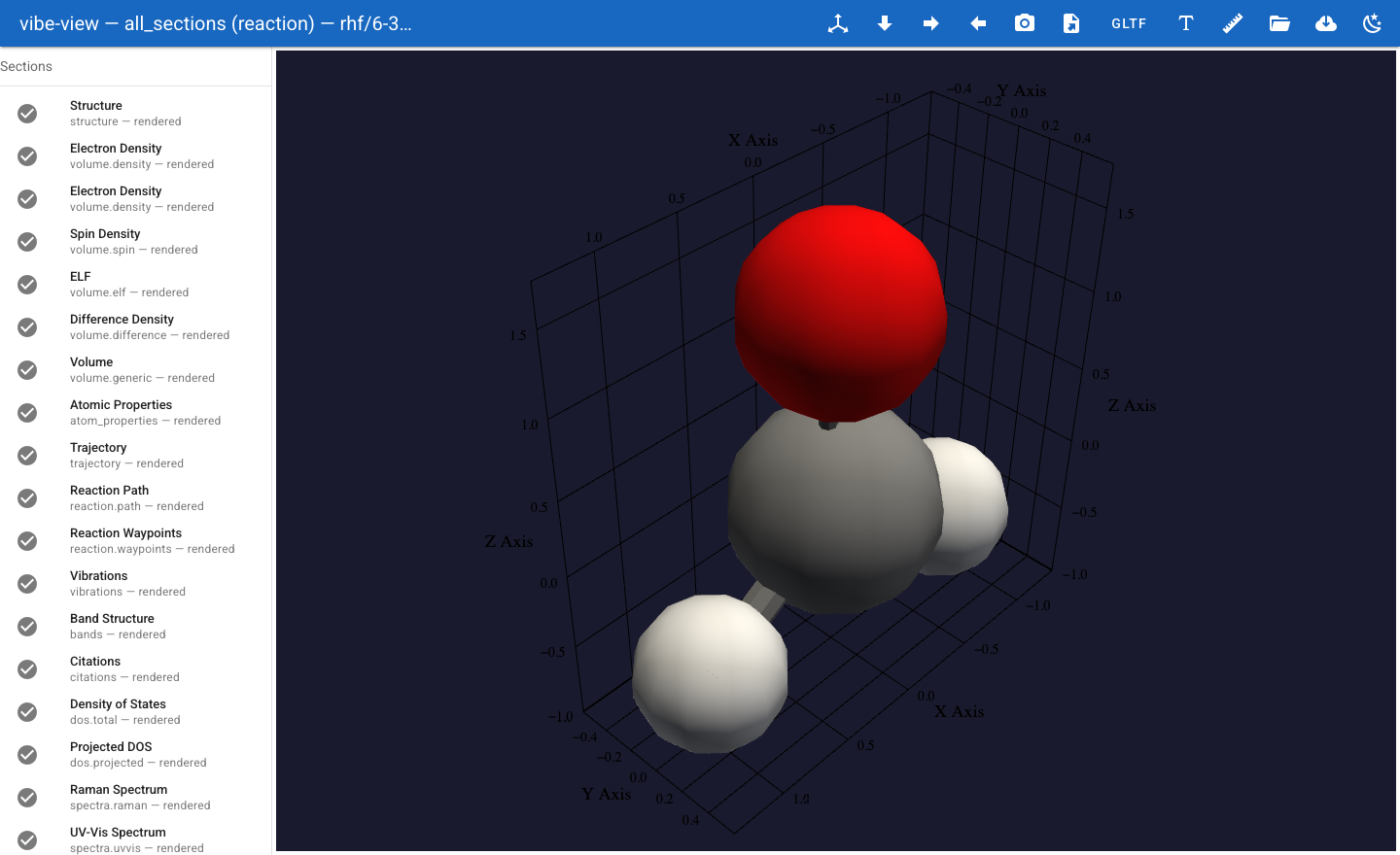
vibe-view open h2o.qvf

Your default browser opens at http://127.0.0.1:8080. You see the water molecule in the 3D viewport with a sidebar listing every section.

Water molecule structure in vibe-view

What happened¶

run_job with output_qvf=True assembled a .qvf archive containing:

Section	Kind	What it shows
`structure`	`structure`	Atom positions, bonds, unit cell (if periodic)
`vol_dens_0`	`volume.density`	SCF electron density as a translucent isosurface
`vol_mo_0`	`volume.orbital`	Highest occupied molecular orbital (HOMO)
`vol_mo_1`	`volume.orbital`	Lowest unoccupied molecular orbital (LUMO)
`wf`	`wavefunction.gto`	Full MO set for on-demand orbital evaluation
`traj0`	`trajectory`	Geometry optimisation frames (from `optimize=True`)
`vib`	`vibrations`	Normal mode animation (from `hessian=True`)
`ir`	`spectra.ir`	IR spectrum (from `hessian=True`)
`props0`	`atom_properties`	Mulliken/Lowdin charges + spin populations
`citations0`	`citations`	BibTeX bundle of every method + basis + library
`scf_hist0`	`scf_history`	Energy + DIIS error convergence charts

Tip

write_cube=["density", "homo", "lumo"] embeds three pre-computed volumetric sections in the QVF. write_molden_file=True embeds the full MO coefficient matrix so vibe-view can evaluate any orbital on demand – far cheaper than writing one cube per orbital. hessian=True adds vibrations, IR spectrum, and thermochemistry; optimize=True adds the geometry optimisation trajectory.

1. Opening QVF files¶

CLI¶

vibe-view open h2o.qvf                    # auto-opens browser at :8080
vibe-view open h2o.qvf --port 9999        # custom port
vibe-view open h2o.qvf --no-browser       # don't open browser
vibe-view open h2o.qvf --host 0.0.0.0    # bind all interfaces (remote access)
vibe-view open nacl.qvf h2co.qvf          # open multiple files -- switch via dropdown

The terminal prints a banner showing every section and its render status:

╔══════════════════════════════════════════════════════════════════════════════╗
║  QVF file: h2o.qvf                                                          ║
║  Source:   vibe-qc 0.15.1.dev0 -- RKS/PBE/6-31G*                            ║
╠══════════════════════════════════════════════════════════════════════════════╣
║  Section ID           Kind                         Status                    ║
╠══════════════════════════════════════════════════════════════════════════════╣
║  structure            structure                    rendered                  ║
║  vol_dens_0           volume.density               rendered                  ║
║  vol_mo_0             volume.orbital               rendered                  ║
║  vol_mo_1             volume.orbital               rendered                  ║
║  wf                   wavefunction.gto             rendered                  ║
║  traj0                trajectory                   rendered                  ║
║  vib                  vibrations                   rendered                  ║
║  ir                   spectra.ir                   rendered                  ║
║  props0               atom_properties              rendered                  ║
║  bond_orders          bond_orders                  rendered                  ║
║  citations0           citations                    rendered                  ║
║  scf_hist0            scf_history                  rendered                  ║
╚══════════════════════════════════════════════════════════════════════════════╝

  12 section(s) will be rendered, 0 skipped, 0 error(s)

In-memory (no disk round-trip)¶

You can pass raw bytes or a BytesIO to avoid writing a .qvf to disk:

import io
from vibeview import launch_qvf

buf = io.BytesIO()
# ... use the QVF writer with buf as the output ...
buf.seek(0)
launch_qvf(buf, open_browser=False)

Remote viewing over SSH¶

ssh -L 8080:127.0.0.1:8080 remote    # port-forward
vibe-view open run.qvf                # run on remote
# open http://127.0.0.1:8080 locally

Table dump¶

Extract tabular data from a QVF without launching the viewer:

vibe-view table h2o.qvf                         # list what's tabulatable
vibe-view table h2o.qvf --kind wavefunction.gto  # MO energies + occupations
vibe-view table h2o.qvf --kind atom_properties   # Mulliken/Lowdin charges
vibe-view table h2o.qvf --kind vibrations        # harmonic frequencies

Output formats:

vibe-view table h2o.qvf --kind wavefunction.gto --format csv   # CSV for spreadsheets
vibe-view table h2o.qvf --kind atom_properties --format json   # JSON for scripts

This is the fastest way to grab frequencies, charges, or MO energies for a paper or a script – no browser, no GUI, just stdout.

Batch rendering¶

Render a whole directory of QVF files into a PNG gallery in one command:

vibe-view batch runs/*.qvf                    # one structure PNG per QVF
vibe-view batch a.qvf -o gallery/             # custom output directory
vibe-view batch *.qvf --size 1200x800         # custom resolution
vibe-view batch a.qvf --volumes               # structure + every volume section

Each QVF’s structure section is rendered offscreen with the dark-theme background and isometric camera. The output directory gets one .png per input file, named {stem}.png. No interactive server starts – this is designed for CI pipelines and scripted comparison galleries.

File info¶

Quickly inspect a QVF without opening the viewer:

vibe-view info h2o.qvf

Prints provenance (method, functional, basis, SCF energy, convergence status, wall time, host), a section-by-section breakdown with member counts and sizes, and the total/archive sizes. Ideal for checking what a QVF contains before opening it, or for logging in automated pipelines.

Fetch from vibe-queue¶

If you use vibe-queue (vq) to run calculations on a cluster, vibe-view from-vq fetches job outputs and opens their QVFs in one step:

vibe-view from-vq abc123                    # fetch and open one job
vibe-view from-vq abc123 def456             # open multiple jobs side by side
vibe-view from-vq abc123 -o ./my-results    # custom fetch directory

This runs vq fetch for each job ID, finds .qvf archives in the fetched workspaces, and launches the viewer. Requires vq installed and on PATH.

Geometry export¶

Extract geometry from a QVF to common formats without opening the viewer:

vibe-view export h2o.qvf -f xyz -o h2o.xyz     # Cartesian coordinates
vibe-view export h2o.qvf -f cif -o h2o.cif     # Crystallographic (periodic)
vibe-view export h2o.qvf -f obj -o h2o.obj     # Wavefront OBJ 3D mesh
vibe-view export h2o.qvf -f gltf -o h2o.gltf   # glTF 2.0 3D exchange format

XYZ and CIF are plain-text; OBJ and glTF are 3D mesh exports suitable for Blender, ParaView, or web-based 3D viewers.

Comparing files¶

Quickly compare two QVFs from the command line:

vibe-view diff hf.qvf pbe.qvf                  # human-readable comparison
vibe-view diff hf.qvf pbe.qvf --json           # machine-readable JSON

Shows energy delta (Eh, kcal/mol, eV), section-kind overlap (which kinds are in both files, which are only in one), geometry RMSD, and SCF convergence status. The --json flag is ideal for automated regression testing.

Machine-readable info¶

For scripting, vibe-view info supports JSON output:

vibe-view info h2o.qvf --json | jq '.scf_energy_eh'   # extract energy
vibe-view info h2o.qvf --json | jq '.sections[].kind'  # list section kinds

2. Complete section-kind reference¶

vibe-view renders all 38 section kinds in the QVF registry. Here is every kind with a brief description:

Structure¶

Kind	What it shows
`structure`	Atoms (CPK colours), bonds, unit cell wireframe if periodic
`structure.symmetry`	Spglib symmetry: space group, Wyckoff positions, operations

Volumetric data¶

Kind	What it shows
`volume.density`	Electron density isosurface (single-sign, positive field)
`volume.orbital`	MO isosurface with signed lobes (blue/red divergent colormap)
`volume.spin`	Spin density – alpha minus beta
`volume.elf`	Electron localisation function
`volume.difference`	Difference density (e.g. SCF minus promolecule)
`volume.potential`	Electrostatic potential mapped onto density isosurface
`volume.rdg`	Reduced density gradient (NCI analysis)
`volume.generic`	Arbitrary scalar field on a grid
`basis.ao`	Atomic orbital isosurface (signed, from GTO evaluation)

Wavefunction¶

Kind	What it shows
`wavefunction.gto`	Full MO set: energy diagram (Grotrian), orbital picker, on-demand evaluation

Electronic structure (periodic)¶

Kind	What it shows
`bands`	Band structure along k-path with Fermi level
`dos.total`	Total density of states
`dos.projected`	Projected DOS (per-atom / per-orbital channels)
`dos.coop`	Crystal Orbital Overlap Population
`dos.cohp`	Crystal Orbital Hamilton Population
`fermi_surface`	Fermi surface in reciprocal space
`phonon_bands`	Phonon dispersion
`phonon_dos`	Phonon density of states
`equation_of_state`	E-V curve with Birch-Murnaghan fit

Spectra¶

Kind	What it shows
`spectra.ir`	Infrared spectrum (stem plot)
`spectra.raman`	Raman spectrum
`spectra.uvvis`	UV/Vis absorption
`spectra.ecd`	Electronic circular dichroism
`spectra.vcd`	Vibrational circular dichroism
`spectra.nmr`	NMR chemical shifts and coupling constants
`spectra.generic`	Arbitrary spectrum (intensity vs frequency)

Dynamics and reactions¶

Kind	What it shows
`trajectory`	Geometry optimisation frames with energy plot
`vibrations`	Normal mode animation with frequency selector
`reaction.path`	Reaction path with per-frame energy + geometry
`reaction.waypoints`	Waypoint markers along a reaction path
`scan.surface`	2D relaxed PES scan as a contour/surface plot

Analysis¶

Kind	What it shows
`atom_properties`	Per-atom charges, spins, populations as an HTML table
`bond_orders`	Mayer/Wiberg bond-order matrix as a table + CSV export
`topology.qtaim`	QTAIM critical points (CP spheres) and bond paths
`citations`	BibTeX reference bundle for the calculation
`scf_history`	SCF convergence: energy + DIIS error per iteration

3. Molecular example: H2O¶

3.1 Structure styles¶

The structure panel offers four rendering styles:

Ball-and-stick (default) – atoms as spheres, bonds as cylinders
Space-filling (CPK) – atoms scaled to van der Waals radii
Wireframe – bonds only, no spheres
Points – atom centres only

Select the style from the dropdown in the structure panel. Ball-and-stick and CPK are best for publication figures.

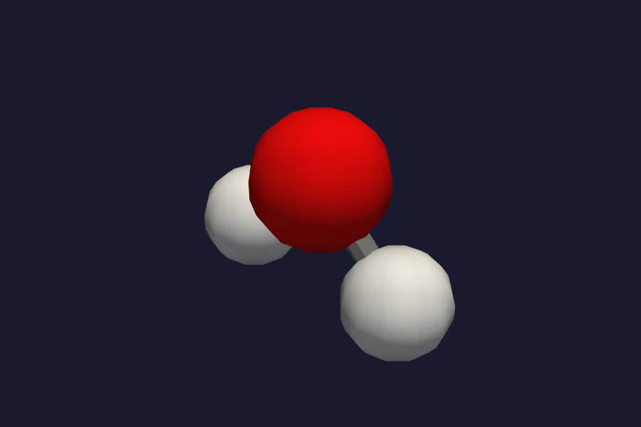
../_images/tutorial-h2o-structure.png — Water molecule in ball-and-stick representation with CPK-coloured atoms.¶

Atom labels can be toggled on/off. For periodic systems the unit-cell wireframe appears automatically and the replication controls (Nx, Ny, Nz) tile atoms, bonds, and any active isosurface together.

Dipole moment arrow¶

When the calculation’s provenance includes a dipole moment vector (in Debye), vibe-view draws an orange arrow from the molecular centroid pointing in the dipole direction. The arrow length is scaled for visibility: 1 D maps to roughly 0.3 A in the viewport. This is automatically shown for any calculation that computes the dipole moment (all SCF methods).

3.2 Electron density¶

Click vol_dens_0 in the sidebar. The viewport overlays a translucent isosurface at the default isovalue of 0.05 e/bohr^3. The sidebar controls let you:

Isovalue – lower values enlarge lobes; higher values squeeze closer to nuclei
Colormap – viridis, plasma, inferno, or custom
Opacity – from fully transparent (0.0) to fully opaque (1.0)

For water, the lone-pair region behind the oxygen is the largest density pocket. At 0.02 e/bohr^3 the density wraps the whole molecule; at 0.1 e/bohr^3 only the core regions near heavy atoms remain.

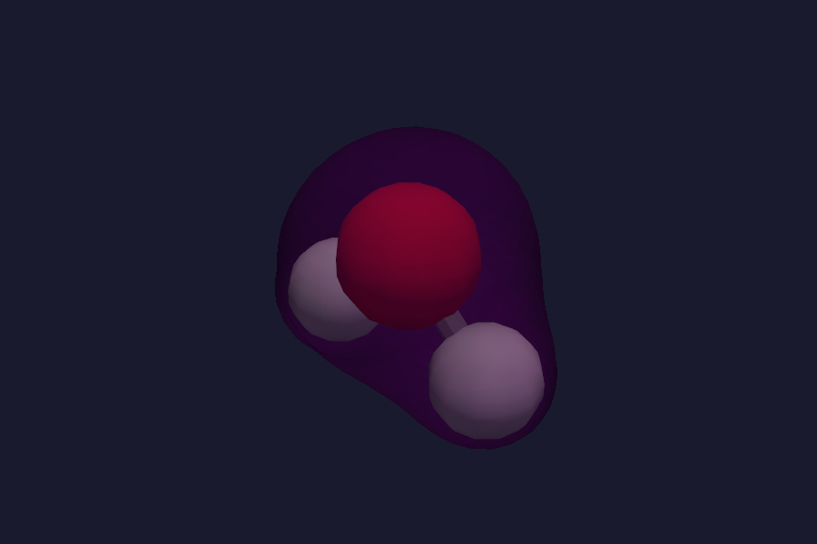
../_images/tutorial-h2o-density.png — Electron density isosurface at 0.05 e/bohr^3, rendered translucent over the ball-and-stick structure.¶

3.3 Molecular orbitals¶

Click vol_mo_0 or vol_mo_1. Because MOs are signed fields, vibe-view uses a divergent colormap: blue for positive lobes, red for negative. The isovalue control works the same way as for density. Typical values for HF-style orbitals: 0.03 -- 0.05 bohr^(-3/2).

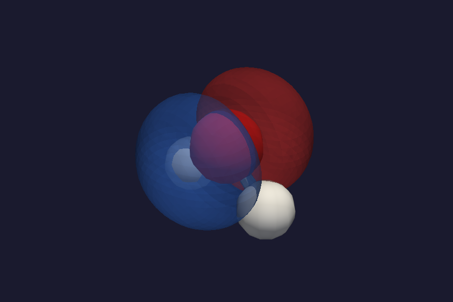
../_images/tutorial-h2o-homo.png — HOMO isosurface with divergent colormap: blue = positive, red = negative.¶

For the full MO set, click wavefunction. The panel shows every MO sorted by energy with:

Occupation number (2.0 for doubly-occupied, 0.0 for virtual)
Energy in Hartree and eV
Symmetry label if the producer wrote them
HOMO/LUMO markers – HOMO is the highest occupied, LUMO the lowest virtual

Click any row to evaluate that orbital on a grid in real time. The grid resolution is configurable:

run_job(
    ...,
    viewer_defaults={"wavefunction": {"grid_spacing": 0.08}},
)

Grotrian diagram¶

The wavefunction panel also includes a Grotrian diagram – an orbital energy level diagram with:

Horizontal bars for each MO at its energy
Occupied levels in a filled colour, virtual in outline
HOMO-LUMO gap clearly visible
Spin-up / spin-down blocks for unrestricted calculations

Click Show Energy Diagram at the bottom of the MO panel to render it.

Orbital animation¶

Click the play button (triangle icon) between the prev/next step buttons to auto-advance through all MOs. The viewer renders each orbital in sequence at 0.5 second intervals. Click pause to stop at the current orbital.

This is useful for:

Scanning the MO manifold for bonding/antibonding character
Finding orbitals with particular spatial features (lone pairs, pi systems)
Recording a screen capture of the orbital sequence

3.4 SCF history¶

Click scf_history. Two stacked charts:

Top: total SCF energy (Hartree) per iteration
Bottom: DIIS error (log scale) per iteration

Hover any point to see exact values. The chart auto-scales both axes; zoom with click-drag.

3.5 Vibrations and IR spectrum¶

With hessian=True in run_job:

vibrations – select a normal mode by frequency (cm^-1). Atoms oscillate along the displacement vectors. The symmetric bend of water is near 1700 cm^-1; symmetric and antisymmetric stretches near 3900 and 4000 cm^-1.
spectra.ir – interactive stem plot of intensity vs frequency. Hover peaks for exact values. Lorentzian broadening is configurable via viewer defaults.

3.6 Geometry-optimisation trajectory¶

With optimize=True:

trajectory – frame-by-frame playback with play/pause/step controls. An energy chart above the viewport shows convergence.

3.7 Citations¶

Click citations for the auto-assembled BibTeX bundle covering every method, functional, basis set, dispersion model, and linked library used in the calculation. Copy-paste ready for papers.

3.8 Thermochemistry¶

When hessian=True is passed to run_job, vibe-qc computes the harmonic vibrational frequencies and appends thermochemistry data to the QVF provenance block. vibe-view surfaces this in the source banner at the top of the window:

ZPVE – zero-point vibrational energy (Eh)
H – thermal enthalpy at the specified temperature/pressure (Eh)
S – entropy in Eh/K
G – Gibbs free energy (Eh)

The default conditions are 298.15 K and 1 atm. To change them:

from vibeqc import ThermoOptions
run_job(mol, ..., hessian=True, thermo_options=ThermoOptions(temperature=500, pressure=2))

The thermochemistry lines appear in the banner together with charge, multiplicity, electron count, and wall time.

3.9 Atom properties¶

Click atom_properties in the sidebar. The viewport switches to an interactive HTML table showing per-atom quantities:

Mulliken charges – default view
Lowdin charges – click the “Lowdin” toggle in the panel header
Spin populations – for open-shell calculations (alpha minus beta)

The table includes a total-charge summary row at the bottom so you can verify at a glance that charges sum to the expected net charge. The charge-kind selector persists across section switches, so you can compare Mulliken vs Lowdin across different molecules without resetting the view.

3.10 MO step browsing¶

When you have a wavefunction.gto section, the orbital picker includes step buttons (prev/next) for rapid browsing. Click the arrows to move through orbitals one at a time without returning to the picker list. Combined with the Grotrian diagram, you can step from HOMO down through occupied orbitals or up from LUMO through virtuals. Use a coarse grid for browsing (grid_spacing=0.15) then switch to fine (0.06) for the final publication-quality view.

3.11 Cube field auto-detection¶

When you import a .cube file directly, vibe-view inspects the cube’s title comment lines to guess the field type. Keywords like “density”, “orbital”, “spin”, “potential”, or “ELF” trigger the appropriate colormap and isovalue defaults automatically. This works for Gaussian, ORCA, and other cube-producing codes.

3.12 Viewer defaults: producer-side hints¶

Control how vibe-view opens your QVF by passing viewer_defaults= to run_job. Hints are embedded in the manifest:

run_job(
    mol, ...,
    viewer_defaults={
        "auto_open": ["vol_dens_0"],
        "vol_dens_0": {"isovalue": 0.02, "colormap": "plasma"},
        "vol_mo_0": {"isovalue": 0.04, "colormap": "RdBu"},
        "wavefunction": {"grid_spacing": 0.08},
    },
)

Supported hints: isovalue, colormap, opacity, grid_spacing, fermi_energy_ev, x_min/x_max, and camera_bookmarks.

4. Periodic example: Si diamond¶

Periodic calculations bring band structure, DOS, replication, and crystal-specific analysis to the viewer.

4.1 Producing the QVF¶

import numpy as np
import vibeqc as vq

# Diamond cubic: two-atom basis, a = 3.567 A
a_bohr = 3.567 / 0.529177
cell = np.eye(3) * a_bohr
frac = np.array([
    [0.00, 0.00, 0.00],
    [0.25, 0.25, 0.25],
])
si = vq.PeriodicSystem(
    3,
    cell,
    [vq.Atom(14, frac[0] @ cell),
     vq.Atom(14, frac[1] @ cell)],
)
basis = vq.BasisSet(si.unit_cell_molecule(), "sto-3g")

# Band path: Gamma-X-W-K-Gamma-L
kpath = vq.kpath_from_segments(
    si,
    segments=[
        ([0.0, 0.0, 0.0], "G", [0.5, 0.0, 0.5], "X"),
        ([0.5, 0.0, 0.5], "X", [0.5, 0.25, 0.75], "W"),
        ([0.5, 0.25, 0.75], "W", [0.375, 0.375, 0.75], "K"),
        ([0.375, 0.375, 0.75], "K", [0.0, 0.0, 0.0], "G"),
        ([0.0, 0.0, 0.0], "G", [0.5, 0.5, 0.5], "L"),
    ],
    points_per_segment=20,
)

vq.run_periodic_job(
    si,
    basis=basis,
    method="RHF",
    output="si-diamond",
    output_qvf=True,
    write_density=True,
    band_structure=vq.band_structure_hcore(si, basis, kpath),
    dos_kmesh=[8, 8, 8],
)

4.2 Structure and replication¶

The structure panel automatically draws the unit-cell wireframe for periodic systems. The sidebar shows replication controls (Nx, Ny, Nz, default 1x1x1). Increase them to tile the cell:

2x2x2 gives an 8-cell supercell – useful for seeing the full bonding environment
3x3x3 is good for publication figures of the lattice

Atoms, bonds, and any active isosurface all tile together.

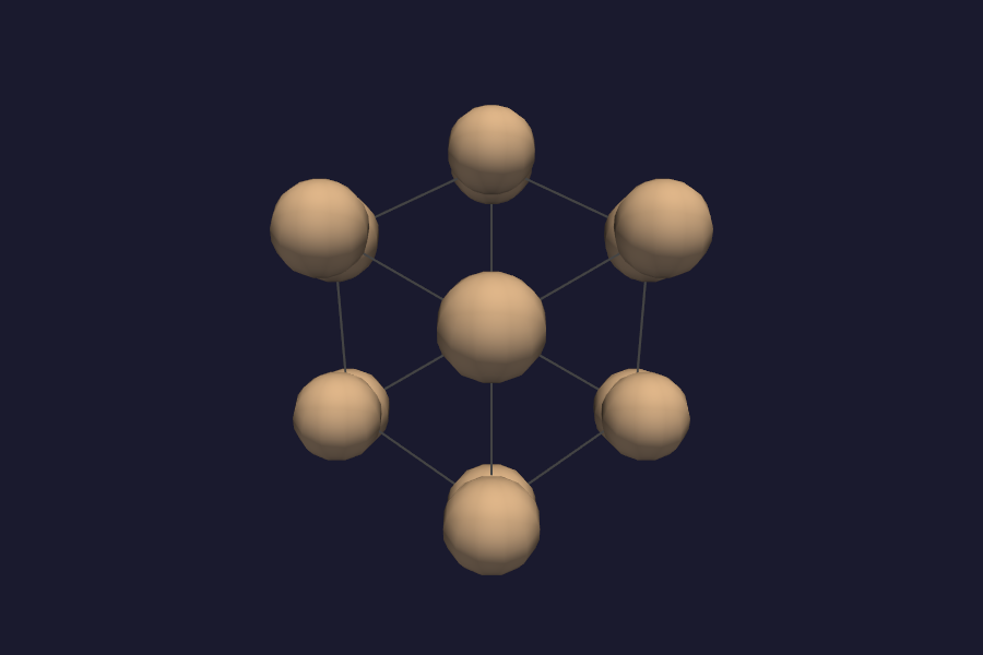
../_images/tutorial-si-structure.png — Si diamond 2x2x2 supercell with unit-cell wireframe.¶

Orbital labelling¶

When a wavefunction.gto section is present, vibe-view labels MOs as Molecular Orbitals. For periodic calculations without GTO wavefunction, the orbitals are labelled as Crystalline Orbitals. The orbital-kind display distinguishes the two in the UI.

MO replication¶

When the structure is replicated (Nx, Ny, Nz > 1), molecular orbitals do not automatically repeat. This is correct: MOs are defined on the unit cell’s atoms. For periodic orbitals, use the volume.orbital section with lattice vectors; vibe-view replicates the isosurface together with the structure.

4.3 Band structure and DOS¶

Click bands. A Plotly chart shows every band’s eigenvalue along the k-path. High-symmetry labels (Gamma, X, W, K, L) mark the segment boundaries. A horizontal dashed line at the Fermi energy (E_F = 0 eV) separates occupied from virtual bands. Hover any band to see its energy.

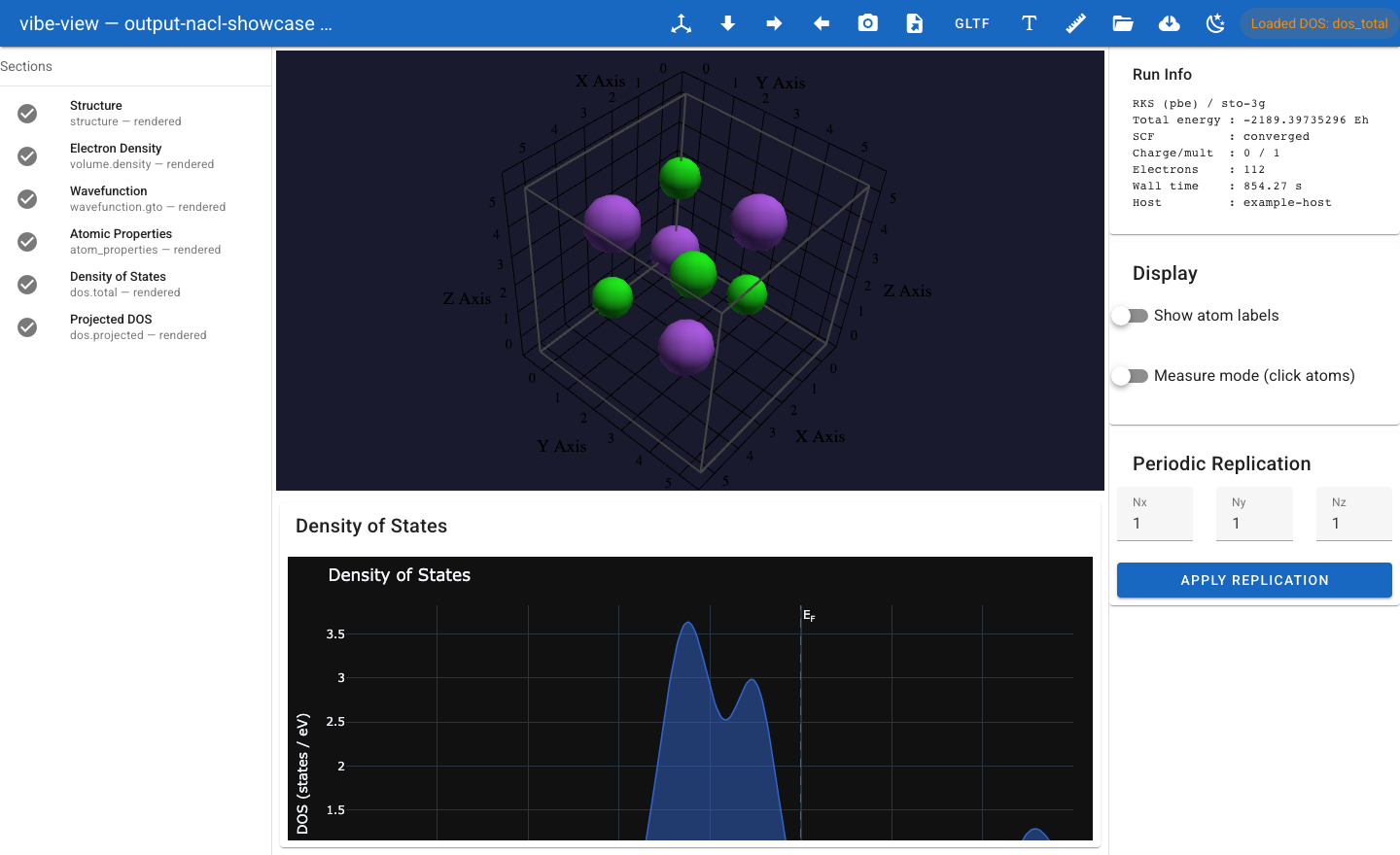
If the QVF has both bands and dos.total, vibe-view draws them as one shared figure on a Fermi-referenced energy axis – the standard solid-state plot. the standard solid-state plot.

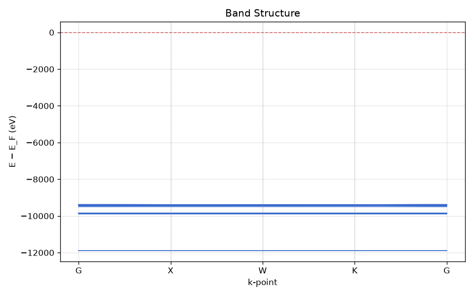
../_images/tutorial-si-bands.png — Si diamond band structure along Gamma-X-W-K-Gamma with Fermi level at 0 eV.¶

Fat bands¶

The dos.projected section enables fat bands – each band line is coloured by its projection onto atomic or orbital channels. The channel legend identifies which colour corresponds to which atom or angular momentum contribution.

vibe-view supports two fat-band renderers:

Matplotlib (PNG via render_to_bytes()) – crisp static output, good for papers
Plotly (interactive HTML) – hover for per-channel values, pan and zoom

COOP / COHP¶

Click dos.coop or dos.cohp for chemical bonding analysis:

COOP (Crystal Orbital Overlap Population) – positive values = bonding, negative = antibonding
COHP (Crystal Orbital Hamilton Population) – negative values = bonding, positive = antibonding (sign-flipped relative to COOP)

The chart shows both the energy-resolved projections and the integrated curve (ICOOP / ICOHP) that gives the net bond order across the energy range.

DOS for periodic system

4.4 Electron density in a crystal¶

Click density. The isosurface tiles with the structure replication, showing how the electron density extends across neighbouring cells. For Si diamond at low isovalues the covalent network is clearly visible; at higher values only the atomic cores remain.

5. Advanced volume features¶

5.1 Electrostatic potential mapping¶

volume.potential sections can be mapped onto a density isosurface – colour the density surface by the ESP value at each vertex. This combines two sections:

Select the volume.density section to show the isosurface
Check “Colour by: potential” in the sidebar controls

The result is an isosurface whose colour encodes the electrostatic potential: red for negative (electron-rich), blue for positive (electron-poor). This is the standard “ESP-mapped density” figure used in computational chemistry papers.

5.2 Multi-isosurface layers¶

You can render multiple isosurfaces at different isovalues simultaneously. In the volume panel, click “Add layer” to add another isosurface contour. Each layer has independent isovalue, colormap, and opacity controls. This is useful for:

Showing core + valence regions of the density
Rendering multiple orbital lobes at different contour levels

5.3 2D cross-section slice¶

The volume panel includes a clip/slice control. Enable it to display a 2D planar slice through the volumetric data at a chosen plane (XY, XZ, YZ, or custom orientation). The slice is rendered as a coloured plane with a scalar bar. Drag the plane position with the slider.

This is useful for inspecting:

Bonding regions in the electron density
Nodal planes in molecular orbitals
ELF basins across a specific plane

5.4 Volume LOD (level of detail)¶

For large volumetric grids (above ~1 million voxels), vibe-view offers a Reduce detail toggle in the volume panel. When enabled, the grid is downsampled before marching cubes, reducing rendering time and memory at the cost of some surface fidelity. The slider controls the downsample factor (2x, 4x, or 8x).

5.5 Spin density¶

volume.spin sections show the difference between alpha and beta electron densities. Like orbitals, this is a signed field: blue for alpha-excess, red for alpha-deficit. This is the key diagnostic for:

Open-shell systems (radicals, transition metals)
Magnetic materials
Broken-symmetry solutions

5.6 ELF (Electron Localisation Function)¶

volume.elf sections visualise electron pair localisation. ELF values range from 0 to 1:

ELF ~ 1: strongly localised pairs (core, lone pairs, covalent bonds)
ELF ~ 0.5: uniform electron gas
ELF ~ 0: region between shells

The default isovalue of 0.8 highlights localisation basins: lone pairs on water’s oxygen, bonding basins between atoms, and core shells.

5.7 NCI (Non-Covalent Interactions)¶

volume.rdg sections carry the Reduced Density Gradient. Combined with a volume.density section, the sign(lambda_2) * rho colouring reveals:

Blue: strong attractive (H-bonds)
Green: van der Waals interactions
Red: steric repulsion

vibe-view’s NCI renderer colours the RDG isosurface (typically at s = 0.5) by the sign(λ2)ρ value, producing the standard NCI plot.

6. Bond analysis¶

6.1 Bond-order matrix¶

When the producer computes bond orders (Mayer or Wiberg), the bond_orders section renders as a triangular matrix table in the viewport. Each cell shows the bond order between two atoms. The table supports:

Colour coding – bond orders colour the structure’s bonds: single bonds in grey, partial double in yellow, double in orange, triple in red.
Legend – a colour bar maps bond order to colour.
CSV export – download the full bond-order matrix as a CSV file.
Sorting – click column headers to sort by bond order.

Bond-order colouring can be toggled in the structure panel.

_static/plots/vibe_view/bond-orders.png — Bond-order matrix table with colour coding. Each cell shows the Mayer/Wiberg bond order between atom pairs.¶

6.2 Periodic bond inference¶

For periodic systems without explicit bond data, vibe-view infers bonds from covalent radii. Atoms within a tolerance (_BOND_TOLERANCE, typically 20% beyond the sum of covalent radii) are connected. The inferred bonds are drawn in the structure viewport and tiled with replication.

Note

Inferred bonds are a visual aid only. For quantitative bond analysis, use bond_orders (Mayer/Wiberg) or topology.qtaim.

6.3 QTAIM critical points and bond paths¶

topology.qtaim sections provide the full topological analysis of the electron density:

Critical points (CPs) rendered as small coloured spheres:
- Red: bond critical points (BCPs) – (3, -1)
- Yellow: ring critical points (RCPs) – (3, +1)
- Green: cage critical points (CCPs) – (3, +3)
- Blue: nuclear critical points (NCPs)
Bond paths drawn as gradient paths connecting nuclei through BCPs.

CPs and bond paths are overlaid on the structure. Click a CP to see its density, Laplacian, and ellipticity at that point.

_static/plots/vibe_view/qtaim.png — QTAIM critical points and bond paths overlaid on the molecular structure.¶

7. Compare and overlay mode¶

vibe-view can open two QVF files side by side or overlay their structures.

Side-by-side¶

vibe-view compare file1.qvf file2.qvf

Two viewports appear side by side. Scroll/rotate in one optionally syncs to the other. Use this to compare:

Two levels of theory (e.g. HF vs PBE density)
Initial vs optimised geometry
Different functionals on the same system

Overlay¶

When comparing, a toggle switches from side-by-side to overlay mode. In overlay mode both structures and both isosurfaces appear in the same viewport, with contrasting colours for the second file (compare highlighting).

Compare highlighting¶

The second file’s atoms and isosurface are rendered in a contrasting colour (magenta by default, configurable). This makes it easy to spot differences:

Geometry: how much did the atoms move?
Density: where did the electron distribution change?
Orbitals: how does the HOMO shift with a different functional?

Density difference¶

When two loaded files both have volume.density sections, the Density Difference card appears in the sidebar. Select File A and File B, then click Show A - B to render the signed density difference (rho_A - rho_B) as a two-colour isosurface:

Blue: electron density accumulation (A > B)
Red: electron density depletion (A < B)

This is the standard difference-density plot used to visualise how electron density redistributes upon bonding, excitation, or changing functional. The isovalue and opacity controls work as usual for the difference field.

Kabsch alignment¶

When two structures have different coordinate frames (e.g. they were optimised starting from different input orientations), the Kabsch least-squares fit automatically aligns them before comparison. This rotates and translates the second structure to minimise the RMSD against the reference, so the residual displacement you see is the genuine geometric difference, not a difference in coordinate frame. The RMSD value is shown in the overlay panel header.

8. Import formats¶

vibe-view can open common structure files directly (no QVF needed). All are auto-detected by extension:

Format	Extension(s)	Notes
QVF	`.qvf`	Native format; all sections
XYZ	`.xyz`	Structure only; auto-detects multi-frame
CIF	`.cif`	Crystallographic; extracts symmetry + cell
Gaussian Cube	`.cube`	Volumetric data; can include multiple datasets
PDB	`.pdb`	Protein Data Bank; residue-based
Mol2	`.mol2`	Tripos format; atom types + bonds
Gaussian input	`.gjf`, `.com`	Extracts geometry + charge/multiplicity
GRO	`.gro`	GROMACS format; box vectors
SDF/Mol	`.sdf`, `.mol`	MDL format; multi-molecule SDF files

vibe-view open molecule.xyz      # open an XYZ file
vibe-view open cell.cif          # open a CIF with symmetry
vibe-view open density.cube      # open a Gaussian cube file

Non-QVF files are treated as having a single structure section (plus volumetric data for .cube files). All the structure controls (styles, labels, replication for CIF) work as usual.

9. Export formats¶

The structure can be exported from vibe-view in four formats:

Format	What it exports	Notes
OBJ	Wavefront OBJ	Mesh export of atoms + bonds for 3D rendering
glTF	glTF 2.0	Standard 3D exchange format, PBR materials
XYZ	XYZ coordinates	Plain-text, multi-atom
CIF	Crystallographic	Fractional coordinates + cell parameters

Export is available from the structure panel’s “Export” dropdown. For CIF export from a molecular geometry, vibe-view wraps the molecule in a box with sufficient vacuum padding.

10. Headless capture API¶

vibe-view includes a headless capture API (vibeview.capture) for generating publication-quality figures from scripts or CI pipelines without opening a browser.

from vibeview.capture import (
    capture_structure,
    capture_volume,
    capture_bands,
    capture_dos,
    capture_scf_history,
    capture_bond_orders,
    capture_spectra,
    capture_energy_diagram,
)
from vibeview.qvf import QVFReader

reader = QVFReader("h2o.qvf")

# 3D structure -- PNG
capture_structure(reader, "fig_structure.png", representation="ball_and_stick")

# Density isosurface with structure context -- PNG
capture_volume(reader, "density", "fig_density.png", isovalue=0.05, colormap="viridis")

# Band structure -- PNG (matplotlib)
capture_bands(reader, "fig_bands.png")

# These produce interactive HTML:
capture_dos(reader, "fig_dos.html")
capture_scf_history(reader, "fig_scf.html")
capture_bond_orders(reader, "fig_bonds.html")
capture_spectra(reader, "fig_ir.html")
capture_energy_diagram(reader, "fig_grotrian.html")

reader.close()

Capture function reference¶

Function	Output	Notes
`capture_structure(reader, path)`	PNG	`representation`, `show_labels`, `replication`
`capture_volume(reader, section_id, path)`	PNG	`isovalue`, `colormap`, `opacity`, `replication`
`capture_bands(reader, path)`	PNG	Auto-detects `bands` section
`capture_dos(reader, path)`	HTML	Auto-detects `dos.total` or `dos.projected`
`capture_scf_history(reader, path)`	HTML	Convergence charts
`capture_bond_orders(reader, path)`	HTML	Bond-order matrix table
`capture_spectra(reader, path)`	HTML	Auto-detects `spectra.*` sections
`capture_energy_diagram(reader, path)`	HTML	Grotrian diagram from `wavefunction.gto`

2D charts (DOS, bands, spectra, SCF history, energy diagram) produce HTML with Plotly or matplotlib. For PNG output of these, convert with a headless browser or use matplotlib’s savefig.

Note

The capture API uses pyvista.Plotter(off_screen=True) and requires no display server. Set PYVISTA_OFF_SCREEN=True in CI environments.

11. QA validation¶

vibe-view includes built-in QA checks for QVF archives. Results appear in the status bar at the bottom of the window.

SCF convergence warnings¶

If the provenance block reports scf_converged: false, vibe-view shows a warning: “SCF did not converge – energies and properties may be unreliable”. This catches unconverged calculations before you spend time analysing meaningless numbers.

Energy sanity checks¶

The viewer checks the total SCF energy for common mistakes:

Positive total energy triggers a warning – this usually means the charge or multiplicity is wrong.
Very large negative energy (below -10 000 Eh) warns about possible basis-set linear dependence, which can happen with diffuse basis sets or tight crystal geometries.

These checks run at file-open time and do not block the view – they are advisory warnings in the status bar.

Isovalue units¶

The volume panel shows the units of the isovalue field in the sidebar: e/bohr^3 for electron density, bohr^(-3/2) for orbitals, dimensionless for ELF. This prevents confusion about what “0.05” means for different field types.

Manifest validation¶

Every .qvf is validated against the QVF JSON Schema on open. Schema violations block the open with a descriptive error. The same validation catches:

Missing required members
Wrong member formats (e.g. binary when JSON expected)
Invalid SHA-256 hashes (verified before every binary read)
Unsupported qvf_version

Critical-section enforcement¶

Sections marked critical: true in the manifest will block the open if vibe-view does not support their kind. This prevents partial renders that would be misleading – a consumer that cannot show a critical section must refuse the entire archive.

12. Tips and gotchas¶

Producer-side hints¶

To control how vibe-view opens a QVF, pass viewer_defaults=:

run_job(
    ...,
    viewer_defaults={
        "auto_open": ["density"],
        "density": {"isovalue": 0.02, "colormap": "plasma", "opacity": 0.5},
        "homo": {"isovalue": 0.04, "colormap": "RdBu"},
        "bands": {"fermi_energy_ev": 0.0},
    },
)

Large grids and memory¶

Volumetric .dat members are lazy-loaded – the binary blob is read from the zip only when you click that section in the UI, not at file-open time. This keeps vibe-view responsive even for multi-gigabyte QVF archives.

For very large grids (> 10^7 voxels), use the “Reduce detail” toggle or pre-set the isovalue to a higher value to reduce the marching-cubes output.

Unsupported sections¶

If the banner reports “skipped, unsupported”, the section kind is not in SUPPORTED_KINDS:

Vendor sections (x_<vendor>.*) are skipped by design
Reserved-but-unwritten kinds are skipped with a hint

Server conflicts¶

If port 8080 is in use, vibe-view open will fail with “port already in use” rather than connecting to a stale server. Use --port 9999 or stop the old server with pkill -f "vibe-view open".

Bookmarks and sessions¶

vibe-view remembers your work across sessions with interactive bookmarks and session save/restore.

Creating a bookmark¶

Set up the view you want: navigate to the right section, adjust isovalue and colormap, rotate/zoom to the best camera angle.
In the Bookmarks card (sidebar, below the section list), type a name like “density-top-view” into the bookmark name field.
Click Save View.

The bookmark captures all five properties: camera position, active section, isovalue, colormap, and opacity. You can save as many bookmarks as you like.

Applying a bookmark¶

Select a saved bookmark from the “My bookmarks” dropdown. vibe-view restores:

The camera to the exact saved position
The active section (switches to it if you were viewing something else)
The isovalue, colormap, and opacity for that section

This is instant – no re-marching, no re-rendering beyond the camera move.

Session save/load¶

A session bundles all your bookmarks plus the current view state into a single .vibe-session JSON file:

{
  "version": 1,
  "active_section": "vol_dens_0",
  "isovalue": 0.05,
  "colormap": "viridis",
  "opacity": 0.6,
  "camera": {"position": [5.0, -3.2, 4.1], "focal_point": [0, 0, 0], ...},
  "replication": [2, 2, 2],
  "user_bookmarks": [
    {"name": "density-top", "camera": {...}, "section_id": "vol_dens_0",
     "isovalue": 0.05, "colormap": "plasma", "opacity": 0.7},
    {"name": "homo-side", "camera": {...}, "section_id": "vol_mo_0",
     "isovalue": 0.04, "colormap": "RdBu", "opacity": 0.6}
  ]
}

Save Session writes this file to disk (default: session.vibe-session, configurable via the path field).
Load Session reads a .vibe-session file and restores the camera, active section, isovalue/colormap/opacity, and all bookmarks.

The path field accepts any writeable location. Sessions are plain JSON and can be shared, version-controlled, or generated by scripts.

Tip

For a presentation or demo, prepare a .vibe-session file with bookmarks for key views (structure overview, density, HOMO, LUMO). Load it at the start and click through the bookmarks for a guided tour of your results.

13. Reaction paths via NEB¶

The Nudged Elastic Band method finds the minimum-energy path (MEP) between a reactant and product. vibe-qc’s run_neb writes a reaction.path section that vibe-view renders as an animated path with per-image energies.

import vibeqc as vq

# NH3 umbrella inversion: planar reactant, inverted product
reactant = vq.Molecule([
    vq.Atom(7, [0.0, 0.0, 0.0]),
    vq.Atom(1, [0.0, 0.94, -0.33]),
    vq.Atom(1, [0.81, -0.47, -0.33]),
    vq.Atom(1, [-0.81, -0.47, -0.33]),
])
product = vq.Molecule([
    vq.Atom(7, [0.0, 0.0, 0.0]),
    vq.Atom(1, [0.0, 0.94, 0.33]),
    vq.Atom(1, [0.81, -0.47, 0.33]),
    vq.Atom(1, [-0.81, -0.47, 0.33]),
])

result = vq.run_neb(reactant, product, basis="sto-3g", method="RHF", n_images=7)
result.write_qvf("nh3-neb")   # writes nh3-neb.qvf

vibe-view open nh3-neb.qvf

In vibe-view, click reaction.path to see the 7 images along the path. The energy profile appears above the viewport; a play/pause strip steps through the images. The transition state (highest-energy image) is highlighted. If the NEB includes a climbing-image phase, that image is marked.

Waypoints (from reaction.waypoints) appear as coloured markers on the energy profile at the reactant, transition state, and product positions.

14. Relaxed PES scan surface¶

A 2D relaxed potential-energy surface scan produces a scan.surface section that vibe-view renders as an interactive 3D surface or contour plot.

Scan surfaces are produced by the QVF output module when the calculation context includes scan_surface data. The vibrator writes this automatically for 2D relaxed scans routed through the output plan API.

# The scan-surface section is written automatically by the output plan
# when a 2D relaxed scan is configured. See docs/tutorial/relaxed_pes_scan.md
# for the full scan workflow.

result = run_job(
    mol,
    ...,
    output_qvf=True,
    # The output plan detects scan data and writes scan.surface
)

The viewport shows a 3D surface (energy vs coordinate 1 vs coordinate 2) with a contour projection on the base plane. Rotate to inspect the energy landscape; hover any grid point to see the energy.

15. NCI and ELF visualization¶

Non-Covalent Interaction (NCI) analysis and the Electron Localisation Function (ELF) are advanced volumetric fields. vibe-view renders them with specialised colour scales: ELF with a hot colormap (0 to 1), and NCI/RDG with the sign(\u03bb2)\u03c1 blue-green-red scale.

These sections are produced through the QVF builder’s context dict. For developers embedding these fields into a QVF:

from vibeqc.output.formats.qvf import qvf_bytes, qvf_density_data

# After an SCF calculation, build a QVF with extra volumetric fields.
# elf_data is a dict of {label: (data_3d, grid_data)}.
# rdg_data is a dict of {label: (rdg_values, sign_lambda2_rho, grid_data)}.

qvf_data = qvf_bytes(
    result, basis_obj, mol,
    density_data=qvf_density_data(result, basis_obj, mol, spacing=0.2),
    elf_data={"elf": (elf_values, elf_grid)},
    rdg_data={"nci": (rdg_values, sl2r_values, nci_grid)},
)
Path("analysis.qvf").write_bytes(qvf_data)

In vibe-view, these appear as volume.elf and volume.rdg sections in the sidebar. Select ELF to see localisation basins (values near 1.0 in warm colours, near 0.5 in cool colours). Select RDG to see the NCI isosurface coloured by sign(\u03bb2)\u03c1 with the density providing context.

Note

The computational routines that produce elf_values and rdg_values from SCF results are being promoted from internal helpers to public API. For the current status, see the QVF consumer reference.

16. Scripted end-to-end workflow¶

Combine vibe-qc, vibe-view table, and the capture API for a fully automated analysis pipeline:

#!/usr/bin/env python3
"""Run a calculation, extract data, and generate figures -- no browser."""
import json, subprocess, sys
from pathlib import Path

from vibeqc import Atom, Molecule, run_job

# 1. Run the calculation
mol = Molecule([
    Atom(8, [0.0, 0.0, 0.0]),
    Atom(1, [0.0, 1.43, -0.98]),
    Atom(1, [0.0, -1.43, -0.98]),
])
run_job(mol, basis="sto-3g", method="rks", functional="PBE",
        output="h2o", output_qvf=True,
        write_cube=["density", "homo", "lumo"],
        write_molden_file=True, hessian=True, optimize=True)

# 2. Extract tabular data (no GUI)
charges = subprocess.run(
    ["vibe-view", "table", "h2o.qvf", "--kind", "atom_properties", "--format", "json"],
    capture_output=True, text=True
)
data = json.loads(charges.stdout)
print(f"Mulliken charges: {[d['mulliken'] for d in data]}")

# 3. Extract MO energies
mo_table = subprocess.run(
    ["vibe-view", "table", "h2o.qvf", "--kind", "wavefunction.gto", "--format", "csv"],
    capture_output=True, text=True
)
Path("h2o-mo-energies.csv").write_text(mo_table.stdout)

# 4. Generate figures via capture API
from vibeview.capture import capture_structure, capture_volume
from vibeview.qvf import QVFReader

reader = QVFReader("h2o.qvf")
capture_structure(reader, "figs/structure.png")
capture_volume(reader, "vol_dens_0", "figs/density.png", isovalue=0.05)
capture_volume(reader, "vol_mo_0", "figs/homo.png", isovalue=0.04, colormap="RdBu")
reader.close()

# 5. Batch PNG gallery of all QVFs in a directory
subprocess.run(["vibe-view", "batch", "runs/*.qvf", "-o", "gallery/"])

print("Pipeline complete: figures in figs/ and gallery/")

This script can run headlessly on a cluster or in CI. The only requirement is PYVISTA_OFF_SCREEN=True for the capture step.

17. Compare mode from CLI¶

Compare two QVF files directly from the command line:

vibe-view compare h2o-hf.qvf h2o-pbe.qvf

Two viewports open side by side. The structures are Kabsch-aligned automatically. Switch to overlay mode with the toggle button to see both structures in one viewport, with the second file highlighted in magenta.

../_images/tutorial-compare-hf.png — HF/STO-3G H2O structure.¶

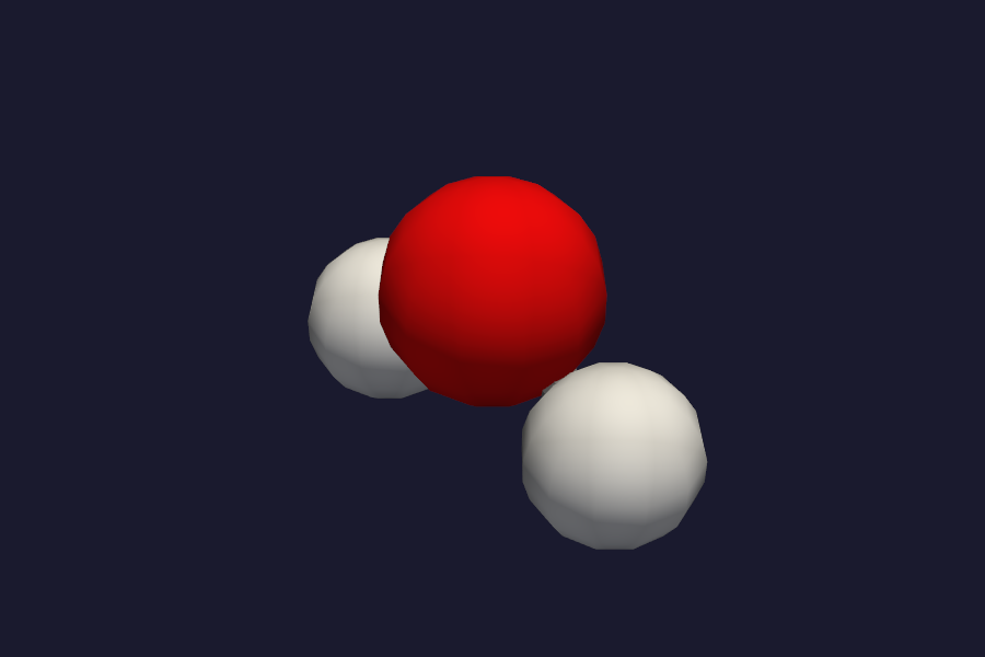
../_images/tutorial-compare-pbe.png — PBE/STO-3G H2O structure – same geometry, different electronic structure. Open both with `vibe-view compare` to see them side by side or overlaid.¶

For a scripted comparison without launching the browser:

from vibeview.qvf import QVFReader
from vibeview.align import kabsch_fit
import numpy as np

r1 = QVFReader("h2o-hf.qvf")
r2 = QVFReader("h2o-pbe.qvf")

s1 = r1.read_structure()
s2 = r2.read_structure()

pos1 = np.array([a.position for a in s1.atoms])
pos2 = np.array([a.position for a in s2.atoms])

aligned, rmsd = kabsch_fit(pos2, pos1)
print(f"RMSD: {rmsd:.4f} A")
print(f"Aligned positions:\n{aligned}")

r1.close()
r2.close()

Next¶

vibe-view user guide: full reference (install routes, programmatic API, every sidebar control).
NEB reaction path: produce reaction.path QVFs with run_neb.
Relaxed PES scan: 2D scan surfaces.
QVF consumer reference: read .qvf files programmatically without launching the viewer.
moltui: the terminal-only sibling viewer for SSH contexts.
auto citations: how the citations section is assembled.
AICCM quickstart: the cyclic cluster model for solids.
Periodic HF: first principles of periodic SCF.

Jupyter integration¶

vibe-view ships a %vibeview line magic for Jupyter notebooks:

%load_ext vibeview.jupyter
%vibeview h2o.qvf                          # structure image + section list
%vibeview h2o.qvf --table atom_properties  # Mulliken/Lowdin charges table
%vibeview h2o.qvf --table wavefunction.gto # MO energies + occupations
%vibeview h2o.qvf --mo                     # same as --table wavefunction.gto
%vibeview h2o.qvf --scf                    # SCF convergence chart (interactive)
%vibeview h2o.qvf --bands                  # band structure plot
%vibeview h2o.qvf --capture density        # density isosurface image
%vibeview h2o.qvf --capture orbital        # orbital isosurface image

Without options, %vibeview shows the structure as an inline PNG, the section list, and key provenance (method, basis, SCF energy, convergence status). All rendering uses the headless capture API under the hood.

Tip

For the full interactive 3D viewer from a notebook, use launch_qvf(reader, open_browser=False) — this starts the Trame server without opening a browser. Connect manually at http://127.0.0.1:8080.

Quick reference¶

Common vibe-qc flags for QVF output¶
Flag	Sections emitted
`output_qvf=True`	structure, atom_properties, citations, scf_history, bond_orders
`write_cube=["density"]`	volume.density
`write_cube=["density","homo","lumo"]`	volume.density, volume.orbital (x2)
`write_molden_file=True`	wavefunction.gto (full MO set)
`hessian=True`	vibrations, spectra.ir, thermochemistry in banner
`optimize=True`	trajectory
`qtaim=True`	topology.qtaim
`band_structure=...`	bands (periodic only)
`dos_kmesh=[8,8,8]`	dos.total, dos.projected (periodic only)
`coop_cohp=True`	dos.coop, dos.cohp (periodic only)
`viewer_defaults={...}`	Embed isovalue/colormap/camera hints