Running in parallel

vibe-qc’s C++ core is OpenMP-parallelised throughout: the four-index ERI evaluation, the SCF commutator-error step, DFT-grid integration, and gradients all distribute across threads on a shared-memory node. For a medium-sized molecule on a modern laptop with 10 cores, expect a 3-6× speed-up over serial.

Two ways to set the thread count

The OpenMP thread count is controllable from two layers: pin it explicitly on the Python call, or set the standard environment variable in the shell. Both are shown below, along with which one wins when both are present.

In Python via run_job

The num_threads= argument on run_job pins the OpenMP thread count for that calculation directly, here a water RKS/PBE single-point at 6-31g* on four threads:

from vibeqc import Molecule, run_job

mol = Molecule.from_xyz("water.xyz")

run_job(
    mol,
    basis="6-31g*",
    method="rks",
    functional="PBE",
    num_threads=4,        # pin the OpenMP thread count
    output="water_pbe",
)

num_threads=None (the default) uses the process-wide default, which follows OMP_NUM_THREADS if set, otherwise falls back to the hardware core count.

At the shell level via OMP_NUM_THREADS

Exporting the standard OMP_NUM_THREADS variable before launching Python sets the thread count for the whole process without touching the job script:

export OMP_NUM_THREADS=4
python3 my_job.py

Shell variables are respected by every vibe-qc entry point and carry through to scripts that invoke run_job, run_rhf, run_rks, run_rhf_periodic_scf, etc., just like in any well-behaved OpenMP code.

If both are set, num_threads= on run_job wins (it calls set_num_threads internally).

What the output shows

The .out file from run_job logs both the active thread count and wall-clock timings for each phase:

  Timings (wall clock, seconds)
  ----------------------------------------------------
  SCF total                               3.421
  SCF avg. per iteration                  0.380  (9 iters)
  Job total                               3.428
  Used 4 OpenMP threads.

Use this to sanity-check that your thread count took effect, and to spot the cost breakdown when iterating on a calculation.

When scaling flattens

OpenMP speed-up plateaus for three reasons:

1. Memory bandwidth dominates the integral loop on larger systems. Beyond ~16 cores the bus saturates and extra threads waste cycles.

2. Fine-grained regions have non-trivial OpenMP overhead. Very small molecules (< 50 basis functions) often run faster at 1-2 threads than at 16 because of parallel-region setup costs.

3. Amdahl’s law. The serial portion, basis-set construction, Fock diagonalisation at each SCF step, doesn’t scale; above 20-30 threads it becomes the bottleneck for moderate-sized systems.

The sweet spot for a 50-200-basis-function calculation on a modern x86 laptop is usually 4-8 threads. For larger jobs (500+ bfs), try the full core count and see if it helps.

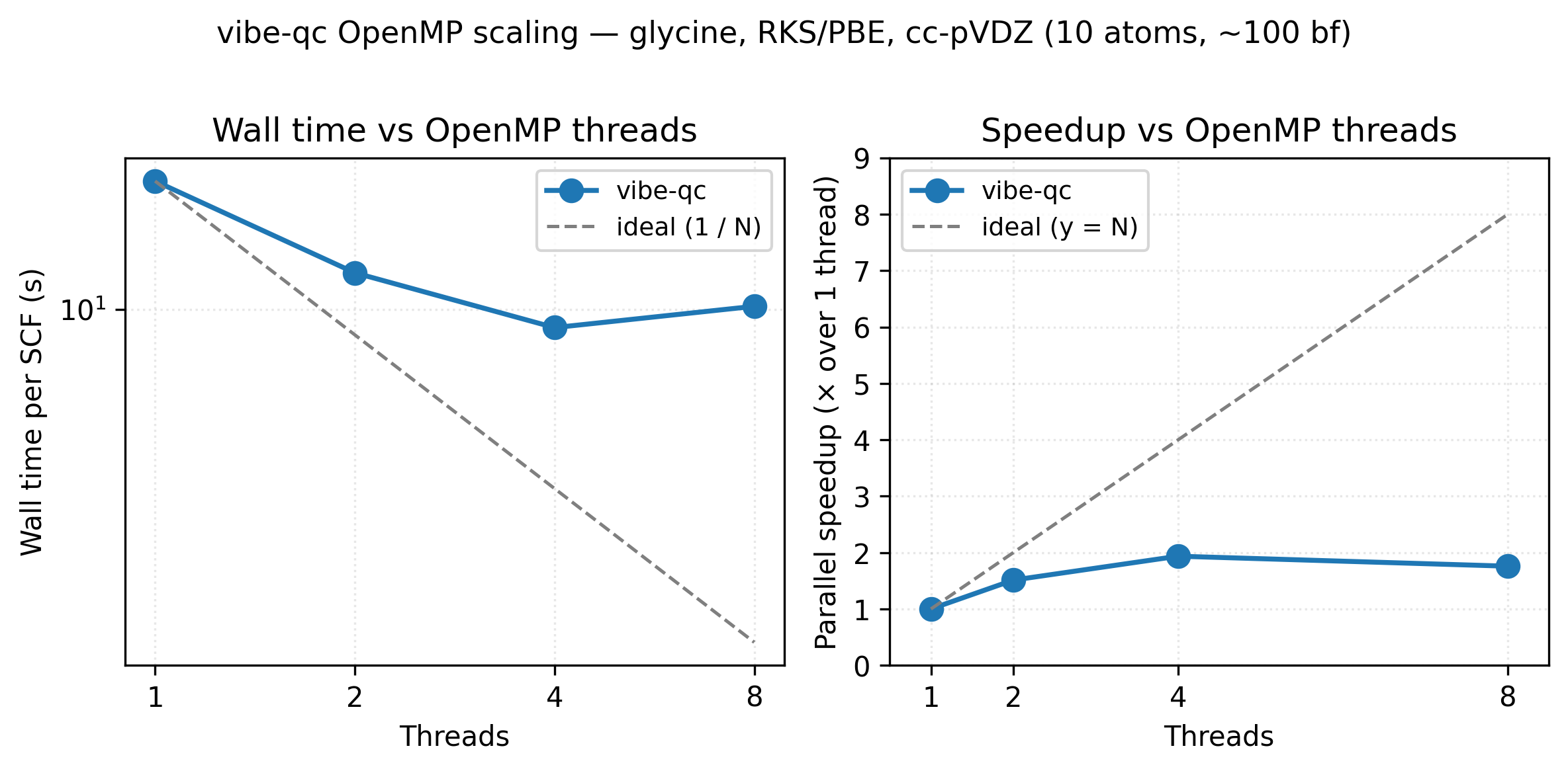
OpenMP scaling for an RKS/PBE single-point on the glycine zwitterion at cc-pVDZ (10 atoms, ~100 basis functions). Going from 1 → 4 threads cuts wall time roughly in half (1.94× speedup); the 8-thread point sits above 4 threads because OpenMP region overhead and Amdahl’s serial floor (basis-set construction, Fock diagonalisation) start to dominate for a system this small. Larger molecules and basis sets keep scaling further before flattening. Reproduce with python3 examples/plots/openmp-scaling.py.

How far each method scales

The 4-8-thread DFT sweet spot above does not transfer to every method. Whether a method scales, and how far, depends on what its hot kernel is: OpenMP work (scales with OMP_NUM_THREADS), a dense BLAS GEMM (scales only if you also raise the BLAS thread count, which vibe-qc pins to 1 by default to avoid oversubscribing the OpenMP regions), or single-threaded Python. The table below is measured wall-clock scaling on a representative system per class; the full data, the OpenMP-vs-BLAS axis decomposition, and a cores-per-job table for batch scheduling live in the repo at benchmarks/openmp_scaling.md.

Method	Scales on	Saturates around	Note
RHF / RKS	OpenMP	~8 (later for large basis)	memory-bandwidth bound, then the serial Eigen eigensolve at very large n
MP2	OpenMP and BLAS	~8 with both axes raised	the one common method that benefits from a threaded BLAS, raise the BLAS vars too
CCSD / CCSD(T)	OpenMP	scales past 16	the threaded scalar intermediate loops dominate wall time, not the single-threaded BLAS ladders
UCCSD	OpenMP	system-size dependent	scalar OpenMP residual loops
CASSCF	OpenMP	active-space dependent	C++ CI sigma build
CASPT2	single-threaded	~1-4	Python numpy contractions, only the SCF underneath threads
TD-DFT	OpenMP (small)	~8	tracks the DFT SCF for small systems, the response build is Python-bound and only dominates for large ones
periodic RKS / UKS	OpenMP inside each k-point	per-k work	the k-point loop is serial, so core count is sized by the per-k Fock/XC cost, not by the number of k-points

Practical guidance for batch runs: give CCSD, CCSD(T) and MP2 the whole node; cap small-molecule DFT, CASPT2 and TD-DFT at a few threads and run several jobs side by side for throughput. For MP2, also set OPENBLAS_NUM_THREADS / VECLIB_MAXIMUM_THREADS to the core count, its dense density-fitting GEMM is the one place a threaded BLAS pays off.

What’s currently parallelised

• ERI evaluation (four-index integrals via libint).

• DFT grid integration (per-atom block split across threads).

• SCF commutator norm \(\lVert \mathbf{F}\mathbf{D}\mathbf{S} - \mathbf{S}\mathbf{D}\mathbf{F} \rVert\).

• Gradient evaluation for HF / DFT / UHF / UKS.

• Periodic lattice sums for overlap / kinetic / nuclear-attraction and ERI contributions.

• Ewald reciprocal-space sums.

What’s not (yet)

• Eigenvalue solves. Single-threaded Eigen SelfAdjointEigenSolver runs. For small systems this doesn’t matter; for very large systems it becomes a bottleneck. Parallel LAPACK integration is tracked on the roadmap.

• Production MPI across nodes. OpenMP is the production shared-memory path today. The optional [mpi] extra provides mpi4py helpers and an experimental GPW z-slab overlay, but normal HF / DFT / MP2 drivers are not distributed across MPI ranks yet. The production strategy is documented in MPI Parallelization.

Performance-checking checklist

If scaling looks wrong, try:

1. Confirm threads are actually used, the .out file’s Used N OpenMP threads line is definitive.

2. Check for Python-side bottlenecks (for-loops, I/O) with a profiler (cProfile). vibe-qc’s C++ side is fast; most surprising slowness comes from the surrounding Python.

3. For periodic calculations, the lattice sum cutoffs grow the parallel work cubically. Too-conservative cutoffs (e.g. cutoff_bohr = 30 for a cell that converges at 12) will cost more than the parallel saves.

4. For DFT, the grid quality affects both wall time and parallel efficiency. n_radial = 75 (default) is usually more efficient than 99 or 120 in absolute wall-clock despite the lower parallelism overhead.

Resources

See the embedded scaling figure: 17.8 s → 9.2 s on 1 → 4 cores for the glycine cc-pVDZ benchmark (Apple M2 baseline). Memory peak scales weakly with thread count, the per-thread engine pool is the dominant overhead and adds <50 MB per additional thread on top of the SCF’s basis-quadratic memory footprint.

References

• OpenMP 5.2 specification. https://www.openmp.org/specifications/. The formal standard for the shared-memory parallelism model used throughout vibe-qc.

• Textbook. T. Rauber and G. Rünger, Parallel Programming, 3rd ed., Springer (2023). Solid general-purpose reference for the algorithmic side of shared-memory parallelism.

• Amdahl’s law. G. M. Amdahl, “Validity of the single-processor approach to achieving large scale computing capabilities,” AFIPS Conf. Proc. 30, 483 (1967). The original argument that bounds parallel speed-up by the serial fraction.

Next

• DFT functional comparison includes a thread-dependent timing snapshot.

• Memory budgeting is a separate concern, see the memory user guide for the pre-flight estimator.