Natural orbitals and the idempotency diagnostic
Canonical molecular orbitals (MOs) are the eigenvectors of the Fock matrix \(\mathbf{F}\). They diagonalize the one-electron Hamiltonian, which makes them the right basis for orbital energies, Koopmans’ ionisation potentials, and SCF convergence.
Natural orbitals (NOs) (Löwdin, Per-Olov (1955). *Quantum Theory of Many-Particle Systems. I. Physical Interpretations by Means of Density Matrices, Natural Spin-Orbitals, and Convergence Problems in the Method of Configurational Interaction.* Physical Review, **97**(6), 1474–1489. doi:[10.1103/PhysRev.97.1474](https://doi.org/10.1103/PhysRev.97.1474)) are eigenvectors of the one-particle reduced density matrix \(\hat\gamma\). They diagonalize the observable, the electron density, which makes them the right basis for population analysis, multireference diagnostics, and any question of the form “where do the electrons actually live?”
For a single Slater determinant the two coincide up to within-subspace rotations. They diverge, informatively, for open-shell, correlated, or symmetry-broken states. This tutorial shows how to compute and read NOs in vibe-qc, and how to interpret the idempotency deviation \(\Delta\) that quantifies the gap between the actual SCF density and a clean single-determinant one.
The basic call
vq.natural_orbitals(result, basis) returns a NaturalOrbitals
dataclass holding occupations and AO-basis NO coefficients, sorted by
descending occupation:
import vibeqc as vq
import numpy as np

mol = vq.Molecule([
    vq.Atom(8, [0.0,  0.00,  0.00]),
    vq.Atom(1, [0.0,  1.43, -0.98]),
    vq.Atom(1, [0.0, -1.43, -0.98]),
])
basis = vq.BasisSet(mol, "6-31g*")

result = vq.run_rhf(mol, basis)
no = vq.natural_orbitals(result, basis)

print(no.occupations[:8])
# [2.0  2.0  2.0  2.0  2.0  ~0  ~0  ~0]   <- exactly five at 2, rest at 0
print(vq.idempotency_deviation(no))
# ~1e-14  <- numerically zero: this is a single Slater determinant
For a closed-shell H₂O / 6-31G* single-determinant SCF the result is
unambiguous: five orbitals at occupation exactly 2.0, the rest at
0.0, and \(\Delta < 10^{-13}\). The NO coefficient matrix is
S-normalized (no.coefficients.T @ S @ no.coefficients == I) and
drop-in compatible with the existing write_cube_mo / Molden
writers, natural orbitals are just another AO-basis MO matrix.
Open-shell: spin natural orbitals
For UHF or UKS, the total NOs (default kind="uhf-total") come from
diagonalizing \(\mathbf{D}_\alpha + \mathbf{D}_\beta\). The
spin NOs (kind="uhf-spin") come from \(\mathbf{D}_\alpha -
\mathbf{D}_\beta\) and have occupations in \([-1, 1]\). The two spin-NOs
with the largest \(|n_i|\) pick out exactly where the unpaired
electrons live.
o2 = vq.Molecule(
    [vq.Atom(8, [0, 0, +1.14]), vq.Atom(8, [0, 0, -1.14])],
    multiplicity=3,                              # ground-state triplet
)
basis_o2 = vq.BasisSet(o2, "6-31g*")
res_o2   = vq.run_uhf(o2, basis_o2)

no_total = vq.natural_orbitals(res_o2, basis_o2, kind="uhf-total")
no_spin  = vq.natural_orbitals(res_o2, basis_o2, kind="uhf-spin")

print(no_total.occupations[:10])
# [2.000 2.000 1.9999 1.9991 ... 1.000 1.000 0.0067]
#                                ^^^^^^^^^^^ two singly-occupied πg*
print(no_spin.occupations[:4])
# [+1.000 +1.000 +0.115 +0.115]
#  ^^^^^^^^^^^^ the two unpaired α electrons in πg*
The leading two spin-NOs have occupations exactly +1: those are the
two unpaired α electrons sitting in the \(\pi_g^*\) pair. Render either
of them with vq.evaluate_ao(basis, points) @ no_spin.coefficients[:, 0]
and you get the textbook \(\pi^*\) shape, the same orbitals chemistry
draws on the back of an envelope, derived directly from the SCF
density.
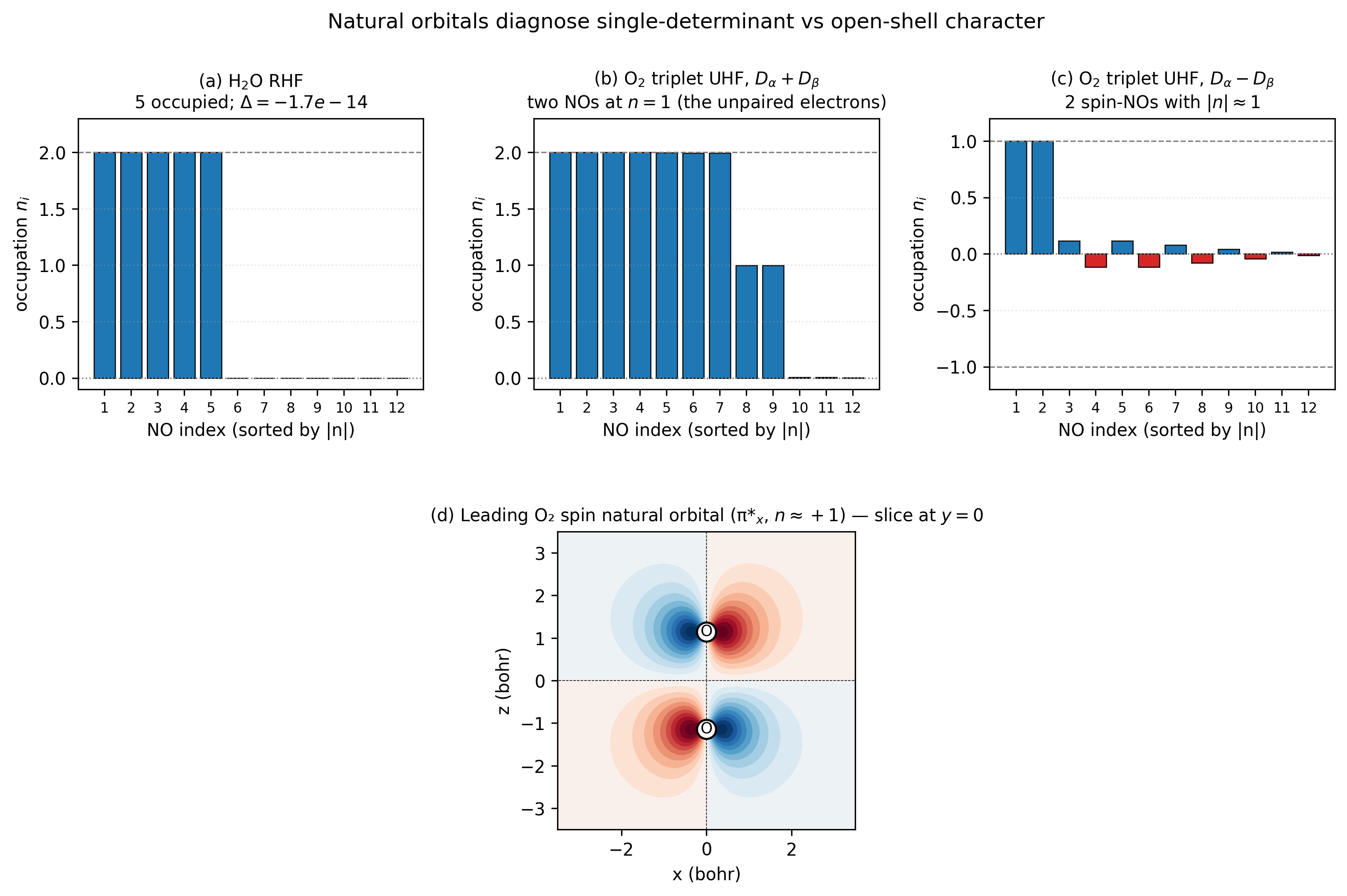
A four-panel anatomy of natural orbitals across the closed-shell /
open-shell boundary. Panel (a) confirms a closed-shell HF state is
genuinely a single determinant, every NO occupation is integer to
machine precision. Panel (b) shows that even for an open-shell
UHF, \(D_\alpha + D_\beta\) has natural occupations clustered at
\(\{0, 1, 2\}\): the two NOs at exactly 1 are the unpaired electrons.
Panel (c) is the same data viewed through the spin density
\(D_\alpha - D_\beta\), only the two unpaired electrons have \(|n_i|
\approx 1\), the rest are spin-polarization tail. Panel (d) plots
the leading spin NO directly: the oxygen \(\pi_g^*\) orbital with a
nodal plane at \(z = 0\) and lobes pointing \(\pm x\) above and below
each O nucleus. Reproduce with
python3 examples/plots/natural-orbital-occupations.py.
Render archived natural orbitals in vibe-view
When a QVF contains a wavefunction.gto section whose orbital_kind is
natural, vibe-view can sample every coefficient row directly. No separate
cube is needed:
vibe-view tui correlated.qvf
Press Tab until the natural-orbital section is active. The terminal UI
renders its default orbital and opens a surface table on the right. Use
Up/Down and Enter to render a selected natural
orbital, or n/p to step through the set. The rows
emphasize occupation rather than a canonical MO energy. When the section
declares occupation_semantics: electron_occupation, D renders the
occupation-weighted total density; i/I adjust the contour.
Natural transition orbitals can use the same archive marker, but their numbers are transition weights rather than electron occupations. The orbital isosurface remains valid, but a weighted sum is not the ground-state electron density. The TUI therefore omits Total density and refuses D for that section. It also refuses density for an older natural section with no semantic marker: individual orbital surfaces remain valid, but the values cannot safely be classified by their sum alone. See Orbital and density visualization for the full terminal workflow.
When NOs differ from canonical MOs
For a single Slater determinant the natural orbitals span the same occupied / virtual subspaces as the canonical MOs, the two sets are related by a within-subspace unitary rotation that the density doesn’t see. NO occupations come out at exactly \(\{0, 2\}\) (or \(\{0, 1\}\) for per-spin UHF), and \(\Delta = 0\) to numerical precision.
For a correlated wavefunction (CASSCF, Roos, Björn O., Taylor, Peter R., and Siegbahn, Per E. M. (1980). *A complete active space SCF method (CASSCF) using a density matrix formulated super-CI approach.* Chemical Physics, **48**(2), 157–173. doi:[10.1016/0301-0104(80)80045-0](https://doi.org/10.1016/0301-0104(80)80045-0); MP2 natural orbitals, DLPNO-CCSD natural orbitals, …) the eigenvalues of \(\hat\gamma\) spread between 0 and 2. Strongly correlated orbitals have occupations near 1 (most informative), weakly correlated ones near 0 or 2. NO occupations are the standard diagnostic for “how much multi-reference character is there?”:
Largest NO occupation \(\ne 2\) |
Interpretation |
|---|---|
\(> 1.95\) |
Single-reference: HF / DFT / single-reference CC are reliable |
\(1.8 \dots 1.95\) |
Mild correlation: MP2 / CCSD usually adequate |
\(1.4 \dots 1.8\) |
Strong correlation: need CASSCF / NEVPT2 / DMRG |
\(\to 1.0\) |
Open-shell singlet / diradical: CASSCF mandatory |
For a single-reference SCF the occupation tail is always at 2 (or 0) to numerical precision; this tutorial’s H₂O example sits at \(2.0\) to 14 digits because the Hartree-Fock density is exactly idempotent. As soon as a correlated method enters, including DLPNO-CCSD(T), which is shipped and covered in DLPNO local correlation, this becomes load-bearing and the spread starts to matter.
Reading \(\Delta\) correctly
The idempotency_deviation formula depends on which density was
diagonalized:
|
\(\Delta\) formula |
What “small \(\Delta\)” means |
|---|---|---|
|
\(\tfrac{1}{2}\sum_i n_i (2 - n_i)\) |
Density is close to a single closed-shell determinant |
|
\(\sum_i n_i (1 - n_i)\) |
Density is close to an idempotent per-spin density (always true for UHF) |
|
\(\tfrac{1}{2}\sum_i (1 - n_i^2)\) |
Mostly a count of basis functions: every spin NO with \(n_i \approx 0\) adds ½, so it is neither a spin-contamination measure nor \(N_{\text{unpaired}}\) |
The triplet-O₂ example has \(\Delta = 1.04\) for uhf-total and
\(\Delta \approx 13\) for uhf-spin. Neither indicates a problem.
\(\Delta_{\text{total}} \approx 1\) comes from the two singly-occupied
NOs each contributing \(\tfrac{1}{2} \cdot 1 \cdot (2 - 1) = 0.5\);
\(\Delta_{\text{spin}} \approx 13\) is close to \((N_\text{bf} - 2)/2\):
O₂/6-31G* has 28 spin NOs, and the 26 besides the two unpaired ones
sit near \(n_i = 0\) and contribute \(\sim 0.5\) each. To recover the
correct \(N_{\text{unpaired}} = 2\) from the spin NOs, count
eigenvalues with \(|n_i| > 0.95\), don’t use the uhf-spin
\(\Delta\). The proper Head-Gordon \(N_{\text{unpaired}}\)
(M. Head-Gordon, Chem. Phys. Lett. 372, 508 (2003),
doi:10.1016/S0009-2614(03)00422-6) is
\(\sum_i \min(n_i, 2 - n_i)\) for the total NOs, equal to 2 for our
O₂.
Theory
The one-particle reduced density matrix is
The electron density is its diagonal: \(\rho(\mathbf{r}) = \gamma(\mathbf{r}, \mathbf{r})\). Löwdin’s 1955 theorem (Löwdin, Per-Olov (1955). *Quantum Theory of Many-Particle Systems. I. Physical Interpretations by Means of Density Matrices, Natural Spin-Orbitals, and Convergence Problems in the Method of Configurational Interaction.* Physical Review, **97**(6), 1474–1489. doi:[10.1103/PhysRev.97.1474](https://doi.org/10.1103/PhysRev.97.1474)) says the operator \(\hat\gamma\) has a complete set of eigenfunctions, the natural orbitals \(\phi_i^{\text{NO}}\), whose eigenvalues \(n_i \in [0, 2]\) (in [0, 1] for spin-orbitals) are the natural occupation numbers:
In a finite AO basis the operator equation becomes the generalised eigenproblem \(\mathbf{D} \mathbf{S} \mathbf{c}_i = n_i \mathbf{c}_i\), which vibe-qc solves via Löwdin’s symmetric route (Löwdin, Per-Olov (1950). *On the Non-Orthogonality Problem Connected with the Use of Atomic Wave Functions in the Theory of Molecules and Crystals.* Journal of Chemical Physics, **18**(3), 365–375. doi:[10.1063/1.1747632](https://doi.org/10.1063/1.1747632)): form \(\tilde{\mathbf{D}} = \mathbf{S}^{1/2} \mathbf{D} \mathbf{S}^{1/2}\), diagonalize, and back-transform. This avoids the non-symmetric eigenproblem \(\mathbf{D} \mathbf{S}\) (its eigenvalues and eigenvectors are real, because \(\mathbf{D}\mathbf{S}\) is similar to the symmetric \(\tilde{\mathbf{D}}\), but a general non-symmetric solver neither exploits that nor returns \(\mathbf{S}\)-orthonormal vectors).
A closed-shell Hartree-Fock density is idempotent in the orthonormal basis up to its occupation factor of 2 (the per-spin density \(\tfrac12 \mathbf{D}\) is idempotent):
That algebraic statement is the statement that \(n_i \in \{0, 2\}\) exactly, every eigenvalue of \(\hat\gamma\) is either fully occupied or fully unoccupied. The deviation \(\Delta = \tfrac{1}{2}\sum_i n_i (2 - n_i)\) is zero iff every \(n_i \in \{0, 2\}\), and grows as occupations drift into the (0, 2) interior. For correlated densities \(\Delta\) is the standard quantitative measure of how much multi-reference character is present.
For UHF, \(\mathbf{D}_\alpha\) and \(\mathbf{D}_\beta\) are each idempotent (in their respective spin spaces) but their sum is not, hence the small “spin polarization” tail in panel (b) above. The spin density \(\mathbf{D}_\alpha - \mathbf{D}_\beta\) has eigenvalues in \([-1, 1]\), and its leading eigenvectors localise the unpaired-electron density. This is the most direct route to “where are the radical centers” without going through the canonical-MO labeling.
Resources
H₂O / 6-31G* RHF + NO diagonalisation: ~25 MB peak RAM, <0.05 s on one core (Apple M2).
O₂ triplet / 6-31G* UHF + total + spin NO + 2D render: ~50 MB peak RAM, <0.5 s on one core.
The full figure (script
[examples/plots/natural-orbital-occupations.py](https://github.com/vibe-qc/vibe-qc/blob/main/examples/plots/natural-orbital-occupations.py)) runs end-to-end in under 1 s. NO diagonalisation cost is \(\mathcal{O}(N_{\text{bf}}^3)\), negligible compared to any SCF.
Caveats
NO sign is arbitrary. Like canonical MOs, NOs are eigenvectors, defined only up to sign. Render the density \(|\phi_i^{\text{NO}}|^2\) if you want a sign-invariant picture.
Within-degenerate-subspace rotations. When two NOs share an occupation (the two \(\pi_g^*\) in O₂ triplet, both at \(n = +1\)), any orthogonal mixture is also a valid pair of NOs. Renderings can legitimately appear “rotated” between runs / packages.
Basis dependence. Like Mulliken / Löwdin charges, NO occupations drift with basis-set size, diffuse functions populate weakly, giving long tails of small-\(n\) NOs. Compare across basis sets only for the leading NOs.
Active-space picking. When NO occupations are used to define a CASSCF active space, the standard rule is “include any NO with \(0.02 < n < 1.98\)” (Pulay, Peter and Hamilton, Tracy P. (1988). *UHF natural orbitals for defining and starting MC-SCF calculations.* Journal of Chemical Physics, **88**(8), 4926–4933. doi:[10.1063/1.454704](https://doi.org/10.1063/1.454704)). vibe-qc ships CASSCF as
run_job(method="casscf", active_space=(...)), and the NO output here is exactly the right input for choosing that active space.
References
Löwdin, P.-O. “Quantum theory of many-particle systems. I. Physical interpretations by means of density matrices, natural spin-orbitals, and convergence problems in the method of configurational interaction,” Phys. Rev. 97, 1474 (1955). The original natural-orbital paper. Defines \(\hat\gamma\), proves the eigenvalue inclusion \(n_i \in [0, 2]\), and introduces the occupation-number diagnostic.
Davidson, E. R. Reduced Density Matrices in Quantum Chemistry. Academic Press (1976). The standard monograph treatment of \(\hat\gamma\) and natural orbitals; the source for most modern multi-reference diagnostics.
McWeeny, R. Methods of Molecular Quantum Mechanics, 2nd ed. Academic Press (1989), Chapter 5. Clearest derivation of the idempotency relation \(\mathbf{D}\mathbf{S}\mathbf{D}\mathbf{S} = \mathbf{D}\mathbf{S}\) and its physical content.
Yamaguchi, K.; Jensen, F.; Dorigo, A.; Houk, K. N. “A spin correction procedure for unrestricted Hartree-Fock and Møller-Plesset wavefunctions for singlet diradicals and polyradicals,” Chem. Phys. Lett. 149, 537 (1988). Origin of the spin-NO contamination diagnostic the
uhf-spinformula approximates.Head-Gordon, M. “Characterizing unpaired electrons from the one-particle density matrix,” Chem. Phys. Lett. 372, 508 (2003). The modern definition of \(N_{\text{unpaired}} = \sum_i \min(n_i, 2 - n_i)\) used in panel-(b)’s “two NOs at \(n = 1\)” reading.
Next
Orbital and density visualization shows how to write the NO coefficients to
.molden/.cubefor external viewers, the NO matrix is drop-in compatible with the same writers.Projected DOS is the periodic-system analogue, energy-resolved decomposition of the density of states onto per-atom orbital projections.