Geometry optimization¶

See also the user-guide reference for the native (ASE-free) optimizer’s full API.

Relax a molecular structure to its energy minimum. vibe-qc uses ASE’s (Larsen, Ask Hjorth, Mortensen, Jens Jørgen, et al. (2017). *The atomic simulation environment - a Python library for working with atoms.* Journal of Physics: Condensed Matter, **29**(27), 273002. doi:[10.1088/1361-648X/aa680e](https://doi.org/10.1088/1361-648X/aa680e)) BFGS-line-search optimizer under the hood, driven by analytic HF/DFT forces from the C++ core. run_job(..., optimize=True) is the one-liner; the standard .out / .molden / .traj files all get written as usual, plus the trajectory animation.

Water at HF/6-31G*¶

Starting from an approximate geometry:

from pathlib import Path
from vibeqc import Atom, Molecule, run_job

mol = Molecule([
    Atom(8, [0.0,   0.0,   0.0  ]),
    Atom(1, [0.0,   1.60, -1.10]),   # slightly off-equilibrium
    Atom(1, [0.0,  -1.60, -1.10]),
])

run_job(
    mol,
    basis="6-31g*",
    method="rhf",
    output="water_opt",
    optimize=True,
    fmax=0.05,            # eV/Å — converged when |F|_max drops below this
    max_opt_steps=50,
)

Files produced:

water_opt.out, initial geometry, optimizer parameters, final optimized geometry, then the full SCF trace at the minimum
water_opt.molden, MOs at the minimum, for Avogadro / Jmol
water_opt.traj, one frame per BFGS step (ASE binary); view with ase gui water_opt.traj

Reading the output¶

After the banner and atom table, water_opt.out contains (vibe-qc 0.17.17 development build):

  Geometry optimization (ASE/BFGS) -> water_opt.traj
  fmax = 0.05 eV/A, max_steps = 50

  Optimized geometry
  Atoms (bohr)
  ------------------------------------------------------------
     1  Z=  8       0.00000000      0.00000000     -0.01145730
     2  Z=  1      -0.00000000      1.42616505     -1.09427135
     3  Z=  1       0.00000000     -1.42616505     -1.09427135
  charge=0  multiplicity=1  n_electrons=10

  iter     energy (Ha)  ...
  (SCF trace at the optimized geometry)
  ...
  converged in 9 iterations; E = -76.0093413306 Ha

The OH bond length and HOH angle at this HF/6-31G* minimum: r(OH) = 0.948 Å, HOH = 105.6° (experimental: 0.957 Å, 104.5°). HF slightly under-shoots the bond and opens the angle.

Parameters¶

The optimization-specific knobs on run_job control the force-convergence target, the optimizer step limit, and how the intermediate SCFs are run:

Argument	Default	Meaning
`fmax`	0.05	Force-convergence tolerance (eV/Å)
`max_opt_steps`	200	Hard iteration limit for the optimizer
`optimizer_backend`	`"auto"`	`"auto"` / `"ase"` / `"native"` / `"brent"`; see user guide
`rhf_options`	`RHFOptions()`	Applied to every intermediate SCF; bump `max_iter` here if BFGS visits hard-to-converge geometries

rhf_options / rks_options forward through to every frame of the optimization, not just the final single point. This matters for H-bonded systems and floppy molecules where one BFGS step sometimes lands on a particularly stubborn geometry, bump max_iter = 200 or add damping = 0.3 to the options struct and the whole trajectory stays stable.

A harder case: the water dimer¶

H-bonded clusters sit on a very flat potential-energy surface, plain BFGS Hessian extrapolation can push the waters apart before the quadratic model is trustworthy. run_job uses BFGSLineSearch which rejects uphill steps by construction, and pair this with a realistic fmax:

from vibeqc import Atom, InitialGuess, Molecule, RHFOptions, run_job

mol = Molecule.from_xyz("h2o_dimer.xyz")  # see examples/h2o_dimer.xyz

rhf_opts = RHFOptions()
rhf_opts.max_iter = 200                   # H-bonded intermediates need it
rhf_opts.initial_guess = InitialGuess.SAD

run_job(
    mol, basis="6-31g*", method="rhf",
    output="water_dimer_opt",
    optimize=True,
    fmax=0.2,                             # loose target for a flat H-bond surface
    max_opt_steps=25,
    rhf_options=rhf_opts,
)

You’ll get R(OO) ≈ 2.98 Å (experimental: 2.976 Å), the well-known HF/6-31G* result. For a real binding-energy number add a correlation method and dispersion; for a chemistry demonstration this is enough.

Visualizing the trajectory¶

ASE’s BFGS converges H₂O at HF/6-31G* in just 4 steps (5 trajectory frames) from a mildly distorted starting geometry. The trajectory below shows the molecule sliding into its equilibrium geometry while the energy drops by ~156 meV:

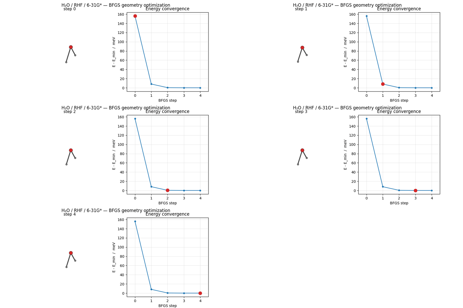
H₂O geometry-optimization animation: 3D ball-and-stick of water relaxing through 4 BFGS steps (5 frames) next to an energy-vs-step plot with a marker tracking the current step.

Regenerated by examples/plots/h2o-opt-trajectory-animation.py from the per-step .traj file. Pattern is the same as the Vibrational frequencies: matplotlib FuncAnimation + PillowWriter, the only difference is that the input here is a series of saved-during-optimization positions rather than displaced-along-mode positions.

The .traj file holds positions, energies, and forces for every frame. ASE’s built-in GUI animates it interactively:

ase gui water_opt.traj

Or inspect programmatically:

import numpy as np
from ase.io import read

frames = read("water_opt.traj", index=":")
energies = np.array([f.get_potential_energy() for f in frames])
print(f"Energy dropped {energies[0] - energies[-1]:.4f} eV over "
      f"{len(frames) - 1} steps")

DFT geometries¶

Same call, different method:

run_job(
    mol, basis="def2-tzvp", method="rks", functional="PBE",
    output="water_pbe_opt",
    optimize=True,
)

PBE lengthens O-H bonds by ~0.02 Å relative to HF and pulls the HOH angle back toward 104°, generally matching experiment more closely (with the well-known caveat that GGA over-binds H-bonds somewhat).

Brent steepest-descent optimizer¶

For systems where the Hessian approximation misbehaves (flat potential energy surfaces, dispersion-bound complexes, near-degenerate states), the Brent steepest-descent backend is a conservative alternative. It never takes an uphill step because every line search is a rigorous 1-D minimisation using Brent’s method (R. P. Brent, Algorithms for Minimization without Derivatives, Prentice-Hall (1973), chapter 5).

from vibeqc import run_job, Atom, Molecule

mol = Molecule([
    Atom(8, [0.0, 0.00, 0.00]),
    Atom(1, [0.0, 1.43, -0.98]),
    Atom(1, [0.0, -1.43, -0.98]),
])

run_job(
    mol,
    basis="6-31g*",
    method="rks",
    functional="PBE",
    dispersion="d3bj",
    optimize=True,
    optimizer_backend="brent",   # steepest-descent + Brent line search
    output="h2o_pbe_brent",
    output_qvf=True,             # write .qvf archive for vibe-view
    fmax=0.05,
)

Open the animation with vibe-view:

vibe-view open h2o_pbe_brent.qvf

The QVF archive carries the full trajectory (per-step geometries and energies), the final density, MO metadata, and the system manifest.

The optimizer summary is printed in .out (vibe-qc 0.17.17 development build):

  Geometry optimization (Brent steepest-descent)
  gtol = 9.72e-04 Ha/bohr, max_steps = 200

  Geometry optimization CONVERGED  (Brent steepest-descent, 3 iterations)
  final max|g| = 6.225e-04 Ha/bohr (threshold 9.723e-04)
  the largest gradient component is within the threshold

A run that stops at max_opt_steps before reaching the threshold prints Geometry optimization NOT CONVERGED instead and ends the job with a GeomOptNotConvergedError; see When the optimizer does not converge in the user guide.

When to use each backend¶

Situation	Recommended backend
Routine organic molecule, tight convergence	ASE BFGS
No ASE installed, frozen-atom constraints	Native L-BFGS-B
Flat PES (H-bonded clusters, vdW complexes)	Brent or ASE BFGS
Near-degenerate states, Hessian misbehaves	Brent
Semi-empirical / MLIP methods	ASE BFGS only (auto-fallback)
`fci`, `nevpt2`, `caspt2`, `mrci`	Native L-BFGS-B or Brent only: ASE (including the `"auto"` default) refuses these with a `ValueError` instead of silently optimizing the mean-field surface (GitLab #357); see the user guide

Theory¶

The sections below build up the machinery behind the one-liner: what a stationary point on the potential-energy surface is, where the analytic forces come from, and how the BFGS line-search optimizer uses them to step toward the minimum.

What “optimization” means on a Born-Oppenheimer PES¶

The Born-Oppenheimer approximation (M. Born and R. Oppenheimer, Ann. Phys. 389, 457 (1927), doi:10.1002/andp.19273892002) decouples nuclear and electronic motion: fix the nuclei at positions \(\mathbf{R} = \{\mathbf{R}_A\}\), solve the electronic Schrödinger equation for those positions, and treat the resulting electronic energy \(E(\mathbf{R})\) as a potential for the nuclei. Geometry optimization is the problem of finding a stationary point on this potential-energy surface (PES):

\[ \mathbf{g}_A \;=\; \frac{\partial E}{\partial \mathbf{R}_A} \;=\; \mathbf{0} \quad \text{for every atom } A. \]

A local minimum has all positive eigenvalues of the Hessian \(\mathbf{H}_{AB} = \partial^2 E / \partial \mathbf{R}_A \partial \mathbf{R}_B\); a transition state has exactly one negative eigenvalue.

The Hellmann-Feynman theorem and analytic forces¶

For a variational electronic method at convergence, the forces \(\mathbf{F}_A = -\mathbf{g}_A\) reduce to expectation values of explicit derivatives of the Hamiltonian:

\[ \mathbf{F}_A \;=\; -\Bigl\langle \Psi \Big| \frac{\partial \hat{H}}{\partial \mathbf{R}_A} \Big| \Psi \Bigr\rangle \;=\; -\frac{\partial E_\text{nuc}}{\partial \mathbf{R}_A} \;+\; \text{electronic terms}. \]

This is the Hellmann-Feynman theorem (Feynman, R. P. (1939). *Forces in Molecules.* Physical Review, **56**(4), 340–343. doi:[10.1103/PhysRev.56.340](https://doi.org/10.1103/PhysRev.56.340)). For an atom-centered Gaussian basis the orbitals themselves move with the nuclei, so the full analytic gradient also needs Pulay forces (Pulay, P. (1969). *Ab initio calculation of force constants and equilibrium geometries in polyatomic molecules. I. Theory.* Molecular Physics, **17**(2), 197–204. doi:[10.1080/00268976900100941](https://doi.org/10.1080/00268976900100941)), corrections from the basis-function derivatives. vibe-qc assembles all the pieces (one-electron derivatives, two-electron ERI derivatives, DFT-grid derivatives for KS, and dispersion-gradient contributions) into an analytic \(\mathbf{g}_A\) at every SCF step. Accuracy is bounded by the SCF tolerance: default settings give forces to a few \(10^{-8}\) Ha/bohr (3 to 4 × \(10^{-8}\) Ha/bohr against a tightly converged SCF for water at HF/6-31G*, vibe-qc 0.17.17 development build).

BFGS: quasi-Newton in quasi-reality¶

A Newton step along the PES would be \(\Delta \mathbf{R} = -\mathbf{H}^{-1} \mathbf{g}\), but computing the Hessian is expensive (the vibrational_frequencies tutorial will do it by finite differences). Quasi-Newton methods build an approximate inverse Hessian \(\mathbf{B}_k\) from the history of steps and gradients. BFGS (Broyden-Fletcher- Goldfarb-Shanno: C. G. Broyden, IMA J. Appl. Math. 6, 76 (1970), doi:10.1093/imamat/6.1.76; R. Fletcher, Comput. J. 13, 317 (1970), doi:10.1093/comjnl/13.3.317; D. Goldfarb, Math. Comp. 24, 23 (1970), doi:10.1090/S0025-5718-1970-0258249-6; D. F. Shanno, Math. Comp. 24, 647 (1970), doi:10.1090/S0025-5718-1970-0274029-X) is the canonical update: given step \(\mathbf{s}_k = \mathbf{R}_{k+1} - \mathbf{R}_k\) and gradient change \(\mathbf{y}_k = \mathbf{g}_{k+1} - \mathbf{g}_k\),

\[ \mathbf{B}_{k+1} = \Bigl( \mathbf{I} - \frac{\mathbf{s}_k \mathbf{y}_k^T}{\mathbf{y}_k^T \mathbf{s}_k} \Bigr) \mathbf{B}_k \Bigl( \mathbf{I} - \frac{\mathbf{y}_k \mathbf{s}_k^T}{\mathbf{y}_k^T \mathbf{s}_k} \Bigr) + \frac{\mathbf{s}_k \mathbf{s}_k^T}{\mathbf{y}_k^T \mathbf{s}_k}. \]

Starting from \(\mathbf{B}_0 = \alpha \mathbf{I}\) (a loose diagonal model), BFGS accumulates curvature information so the quadratic model becomes genuinely predictive near the minimum.

The line-search variant used here¶

vibe-qc’s run_job(..., optimize=True) actually runs ASE’s BFGSLineSearch, not bare BFGS. The line search enforces the Wolfe conditions (P. Wolfe, SIAM Rev. 11, 226 (1969), doi:10.1137/1011036), sufficient-decrease plus curvature, on each step, so every accepted move reduces the energy. This matters on flat / weakly-bound surfaces (H-bonded clusters, van-der-Waals complexes) where plain BFGS’s quadratic model sometimes predicts wild steps that blow the system apart; the line search catches them. Cost: 1-3 extra SCFs per BFGS step when the first trial step is uphill.

Convergence criteria¶

vibe-qc stops when the maximum-component force is below fmax (units eV/Å, ASE convention). Default fmax = 0.05 is “medium-tight” (~1 × 10⁻³ Ha/bohr). Benchmark-quality geometries use fmax = 0.01; flat H-bonded clusters are often given a looser fmax = 0.2 for a first pass, because tighter targets cost many more steps on such a surface.

Resources¶

~150 MB peak RAM, ~5 s on one core (Apple M2 baseline) for the H₂O example: 4 BFGSLineSearch steps (5 trajectory frames), each one HF/6-31G* + analytic gradient. The water-trimer optimization in examples/molecular/input-h2o-trimer-opt.py is ~5 minutes, basis size and step count both grow with system size.

References¶

Born-Oppenheimer approximation. M. Born and J. R. Oppenheimer, “Zur Quantentheorie der Molekeln,” Ann. Phys. 389, 457 (1927).
Hellmann-Feynman theorem. H. Hellmann, Einführung in die Quantenchemie, Deuticke (1937); R. P. Feynman, “Forces in molecules,” Phys. Rev. 56, 340 (1939).
Pulay forces. P. Pulay, “Ab initio calculation of force constants and equilibrium geometries in polyatomic molecules. I. Theory,” Mol. Phys. 17, 197 (1969).
BFGS update. C. G. Broyden, “The convergence of a class of double-rank minimization algorithms,” IMA J. Appl. Math. 6, 76 (1970) and parallel papers by Fletcher, Goldfarb, Shanno (1970). Textbook treatment: J. Nocedal and S. J. Wright, Numerical Optimization, 2nd ed., Springer (2006), chapters 6-8.
Wolfe conditions / line search. P. Wolfe, “Convergence conditions for ascent methods,” SIAM Review 11, 226 (1969).
ASE (the driver). A. H. Larsen et al., “The atomic simulation environment, a Python library for working with atoms,” J. Phys. Condens. Matter 29, 273002 (2017).

Next¶

Post-SCF analysis, charges, bond orders, and dipole moment at the optimized geometry.
Vibrational frequencies, once the geometry is at a stationary point, compute the Hessian to classify it.