Projected density of states (PDOS)¶

A total density of states tells you how many states occur near an energy. A projected density of states estimates which atoms and angular-momentum channels contribute to those states. In an LCAO code such as vibe-qc, the default projection is a Mulliken partition of every Bloch orbital over the AO basis.

This tutorial separates two workflows that should not be confused:

Workflow	Operator	Use
`density_of_states_projected_hcore`	kinetic plus nuclear attraction	teaching, AO-label checks, fast qualitative survey
`run_periodic_job(..., output_qvf=True)`	route-dependent post-SCF reconstruction	diagnostic QVF output; verify the operator before scientific interpretation

Hcore contains no Coulomb, exchange, or exchange-correlation potential. Its orbital character can differ from a self-consistent result. Label every Hcore plot explicitly and do not report its gap as a Hartree-Fock or DFT prediction.

A complete Hcore example¶

The following example creates a 1D LiH chain, verifies the AO partition, computes an atom and angular-momentum projected DOS, compares it with a separately computed total DOS, and writes a plot:

import numpy as np
import vibeqc as vq
from vibeqc.plot import pdos_figure

a = 5.5
system = vq.PeriodicSystem(
    dim=1,
    lattice=[[a, 0.0, 0.0], [0.0, 30.0, 0.0], [0.0, 0.0, 30.0]],
    unit_cell=[
        vq.Atom(3, [0.0, 0.0, 0.0]),
        vq.Atom(1, [0.5 * a, 0.0, 0.0]),
    ],
)
basis = vq.BasisSet(system.unit_cell_molecule(), "sto-3g")

groups = vq.ao_groups_per_atom_l(system, basis)
assigned = [ao for indices in groups.values() for ao in indices]
if len(assigned) != len(set(assigned)) or sorted(assigned) != list(range(basis.nbasis)):
    raise ValueError("PDOS groups must partition every AO exactly once")

pdos = vq.density_of_states_projected_hcore(
    system,
    basis,
    mesh=[200, 1, 1],
    projection=groups,
    sigma=0.005,
    n_electrons_per_cell=4,
)
dos = vq.density_of_states_hcore(
    system,
    basis,
    mesh=[200, 1, 1],
    sigma=0.005,
    n_electrons_per_cell=4,
)

print(pdos.group_labels)
print("maximum projected-total error:", np.max(np.abs(pdos.total - dos.dos)))

fig = pdos_figure(pdos, title="LiH chain (STO-3G, Hcore PDOS)")
fig.savefig("lih-chain-hcore-pdos.png", dpi=180)

pdos.energies, pdos.total, and each contribution array have the same length. Energies and sigma are in Hartree. The plotting layer displays eV by default and can shift the reference energy to pdos.e_fermi.

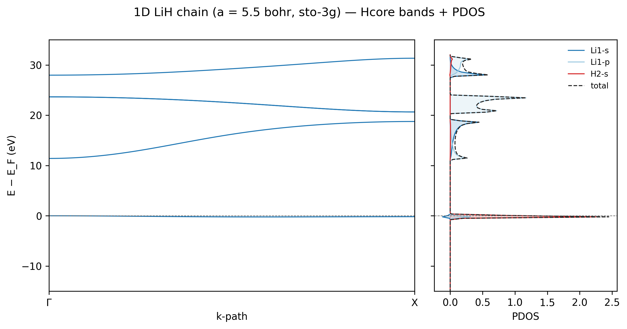
Bands and PDOS for a 1D LiH Hcore example. The plot is a teaching illustration of Mulliken channel weights, not a self-consistent band prediction.

The figure is useful for learning how Li-s, Li-p, and H-s channels are shown. The chemical interpretation remains qualitative because this example uses Hcore. Reproduce the maintained plot with examples/plots/lih-chain-pdos.py.

The projection equation¶

At each k point, vibe-qc solves the generalized eigenproblem

\[ \mathbf{F}(\mathbf{k})\mathbf{C}_n(\mathbf{k}) =\varepsilon_n(\mathbf{k}) \mathbf{S}(\mathbf{k})\mathbf{C}_n(\mathbf{k}), \]

with normalized eigenvectors,

\[ \mathbf{C}_n^\dagger(\mathbf{k}) \mathbf{S}(\mathbf{k})\mathbf{C}_m(\mathbf{k})=\delta_{nm}. \]

The Mulliken weight of AO \(\mu\) in band \(n\) is

\[ p_{\mu n\mathbf{k}}= \operatorname{Re}\left[ C^*_{\mu n}(\mathbf{k}) \left(\mathbf{S}(\mathbf{k})\mathbf{C}_n(\mathbf{k})\right)_\mu \right]. \]

Normalization gives

\[ \sum_\mu p_{\mu n\mathbf{k}}=1. \]

For a group \(A\) containing selected AO indices, the broadened PDOS is

\[ g_A(E)=\sum_\mathbf{k}w_\mathbf{k}\sum_n \left(\sum_{\mu\in A}p_{\mu n\mathbf{k}}\right) \frac{\exp[-(E-\varepsilon_{n\mathbf{k}})^2/(2\sigma^2)]} {\sqrt{2\pi}\sigma}, \]

where \(\sum_\mathbf{k}w_\mathbf{k}=1\). If the groups form a complete, non-overlapping AO partition, their curves sum to the independently computed total DOS at every energy. ProjectedDensityOfStates.total itself is built by adding the requested group curves, so comparing those curves with that member is tautological. Validate the AO indices first, then compare against a separate unprojected DOS evaluated with the same operator, mesh, grid, and broadening.

Individual Mulliken weights can be negative because overlap populations can be negative. This is not by itself an error. Interpret robust group sums and trends, not one isolated AO coefficient.

Choose projection groups¶

The Hcore convenience function accepts:

`projection`	Channels
`"atoms"`	one channel per atom
`"atoms_l"`	atom and angular momentum, such as `O1-p`
dictionary	explicit label to AO-index mapping

For an explicit real-space Fock/overlap workflow, use vq.ao_groups_per_atom(system, basis) or vq.ao_groups_per_atom_l(system, basis) to build a complete partition. A custom selection can be passed to the lower-level function:

import vibeqc as vq


def project_selected_aos(fock_real, overlap_real, kmesh):
    groups = {
        "metal_d": [10, 11, 12, 13, 14],
        "ligand_p": [25, 26, 27],
    }
    return vq.density_of_states_projected(
        fock_real,
        overlap_real,
        kmesh,
        groups=groups,
        sigma=0.005,
    )

Hard-coded AO indices are fragile when the basis changes. Record the basis and print the generated standard groups before creating a custom partition.

Changing the groups does not change the underlying Mulliken rule. A Bader, IAO, or Wannier analysis is a different projection method and should not be described as a custom Mulliken grouping.

PDOS diagnostics in a QVF¶

For a converged Gaussian-basis periodic calculation, run_periodic_job reconstructs a post-SCF operator, computes total DOS and atom/angular-momentum PDOS, and embeds both in the default QVF archive. Control the post-SCF mesh with dos_kmesh:

import vibeqc as vq


def run_bulk_with_pdos(system, basis):
    return vq.run_periodic_job(
        system,
        basis,
        method="RKS",
        functional="pbe",
        kpoints=[4, 4, 4],
        dos_kmesh=[12, 12, 12],
        output_qvf=True,
        output="output-bulk-pbe",
    )

Open output-bulk-pbe.qvf in vibe-view and select the DOS or PDOS section. The QVF spectrum uses a 0.05 eV Gaussian width. The DOS mesh is separate from the SCF mesh and needs its own convergence study. Use shapes consistent with dimensionality, such as [64, 1, 1] for a 1D chain or [24, 24, 1] for a 2D sheet.

For RKS and UKS, this current QVF reconstruction omits the exchange-correlation potential; the restricted path also applies full exact exchange. It is not the converged Kohn-Sham operator. Use these curves as diagnostics only, and use a route-specific converged-operator helper for a quantitative DFT PDOS claim.

The lower-level density_of_states_projected entry point consumes explicit real-space LatticeMatrixSet Fock and overlap objects. Generic periodic result objects do not promise fock_real or overlap_real attributes. Do not copy older examples that assume those fields exist. Route-specific spectrum helpers are listed in Band structure and DOS.

Converge a PDOS¶

Use this order so one numerical effect is not hidden by another:

Converge the physical SCF result with respect to basis, Coulomb route, SCF k mesh, and numerical thresholds.
Increase the DOS mesh until peak positions and integrated channel weights stop changing at the accuracy relevant to the claim.
Choose sigma small enough to retain resolved features but large enough to display the converged mesh smoothly.
Repeat the projection with a second reasonable basis when the chemical conclusion depends on a small difference between channels.
Verify that the groups partition every AO exactly once, then compare their sum with a separately computed unprojected DOS on the identical grid.
Retain the input, .out, .system, .qvf, basis identity, and citations.

A large sigma can make an under-sampled mesh look smooth. Smoothness is not evidence of k-point convergence.

CPU time and memory¶

For \(N_\mathbf{k}\) k points and \(N_\mathrm{bf}\) basis functions, the leading diagonalization trend is

\[ T\sim\mathcal{O}(N_\mathbf{k}N_\mathrm{bf}^3). \]

Each k-point diagonalization needs matrix workspace near \(\mathcal{O}(N_\mathrm{bf}^2)\). The current implementation retains Mulliken weights of shape \((N_\mathbf{k},N_\mathrm{bf},N_\mathrm{bf})\), so PDOS working memory scales as \(\mathcal{O}(N_\mathbf{k}N_\mathrm{bf}^2)\). Stored curves add \(\mathcal{O}(GN_E)\) for \(G\) groups and \(N_E\) energy points. The preceding SCF can still set the process peak, while a dense PDOS mesh can dominate post-processing CPU time.

Record CPU time, wall time, peak RSS, basis count, SCF mesh, PDOS mesh, energy-grid size, group count, spin treatment, and sigma together.

Interpretation limits¶

Mulliken projections are basis dependent, especially with diffuse or highly redundant basis functions. Use them primarily for trends and broad orbital character.
Hcore PDOS is qualitative. Electron-electron interactions can alter band ordering and character even when the Hcore picture looks plausible.
Negative channel values can arise from non-orthogonal overlap populations.
Integer n_electrons_per_cell filling supplies a plotting reference, not a finite-temperature chemical potential. Metals require converged k-point sampling, occupations, smearing temperature, entropy, and energy convention.
A PDOS identifies basis-function character, not oxidation state or uniquely assigned charge. Combine it with real-space density, bond analysis, and chemical context.

References and next steps¶

The Mulliken population definition originates with R. S. Mulliken, J. Chem. Phys. 23, 1833 (1955). For the broader chemical interpretation of bands and DOS in extended systems, see R. Hoffmann, Solids and Surfaces: A Chemist’s View of Bonding in Extended Structures (1988).

Continue with:

Band structure and DOS for path versus mesh sampling, Gaussian normalization, route-specific SCF helpers, and resource scaling.
Periodic orbital cubes for the spatial view of a selected Bloch orbital.
Smearing for metals and fractional occupations.