Peierls dimerisation of a 1D H-chain

A uniform 1D chain of hydrogen atoms, equally spaced, has a half-filled band that crosses the Fermi level at \(k = \pi / 2a\), a 1D metal. Peierls (1955) showed that any 1D metal is thermodynamically unstable against a periodic lattice distortion that doubles the unit cell: pairs of atoms move together, opening a gap at the folded-back band edge and lowering the total energy. This tutorial traces that instability directly by scanning the dimerisation amplitude and watching the total energy fall.

The scan

Start from a two-atom unit cell with atoms at \(0\) and \(a/2\) (uniform spacing) and shift the second atom by \(-\delta\) along the chain:

• Uniform: \(\delta = 0\). Both H-H distances equal \(a/2\).

• Dimerised: \(\delta > 0\). Short bond \(a/2 - \delta\); long bond \(a/2 + \delta\).

The complete scan is in examples/periodic/input-h-chain-peierls.py; the minimal excerpt:

The chain is a dim=3 cell with vacuum on the two transverse axes and a k mesh along the chain only. vibe-qc has no route with a consistent 1-D Coulomb gauge, so a PeriodicSystem(dim=1, ...) cannot be run with GDF (Sun, Qiming, Berkelbach, Timothy C., et al. (2017). *Gaussian and plane-wave mixed density fitting for periodic systems.* Journal of Chemical Physics, **147**(16), 164119. doi:[10.1063/1.4998644](https://doi.org/10.1063/1.4998644)); the vacuum box is the supported way to sample k along a wire, and the vacuum PAD is part of the model.

import numpy as np
from vibeqc import (
    Atom, BasisSet, PeriodicRHFOptions, PeriodicSystem,
    run_krhf_periodic_gdf,
)

A = 5.0                          # lattice parameter (bohr)
PAD = 15.0                       # transverse vacuum (bohr)
KMESH = (8, 1, 1)

def build_system(delta: float) -> PeriodicSystem:
    lattice = np.diag([A, PAD, PAD])
    unit_cell = [
        Atom(1, [0.0,              0.0, 0.0]),
        Atom(1, [A / 2.0 - delta,  0.0, 0.0]),
    ]
    return PeriodicSystem(dim=3, lattice=lattice, unit_cell=unit_cell)

opts = PeriodicRHFOptions()
opts.conv_tol_energy = 1e-8
opts.conv_tol_grad = 1e-3        # see caveat below
opts.max_iter = 80

for delta in (0.0, 0.2, 0.4, 0.6, 0.8, 1.0, 1.1):
    sysp = build_system(delta)
    basis = BasisSet(sysp.unit_cell_molecule(), "pob-tzvp")
    r = run_krhf_periodic_gdf(sysp, basis, KMESH, opts, progress=False)
    short, long = A/2 - delta, A/2 + delta
    print(f"δ={delta:.2f}  R_short={short:.3f}  R_long={long:.3f}  "
          f"E={r.energy:.6f}  ({'yes' if r.converged else 'NO'})")

Output of the example (vibe-qc 0.17.14):

δ=0.00  R_short=2.500  R_long=2.500  E=-1.029634  (yes)
δ=0.20  R_short=2.300  R_long=2.700  E=-1.049378  (yes)
δ=0.40  R_short=2.100  R_long=2.900  E=-1.071390  (yes)
δ=0.60  R_short=1.900  R_long=3.100  E=-1.093370  (yes)
δ=0.80  R_short=1.700  R_long=3.300  E=-1.112883  (yes)
δ=1.00  R_short=1.500  R_long=3.500  E=-1.126474  (yes)
δ=1.10  R_short=1.400  R_long=3.600  E=-1.129363  (yes)

As soon as the short bond shortens below the uniform spacing, the energy drops monotonically. At \(\delta = 1.1\) (short bond \(= 1.4\) bohr, exactly the isolated H₂ equilibrium) the energy has fallen by 0.0997 Ha per unit cell from the uniform case. That’s ~2.7 eV, a large, unambiguous stabilisation.

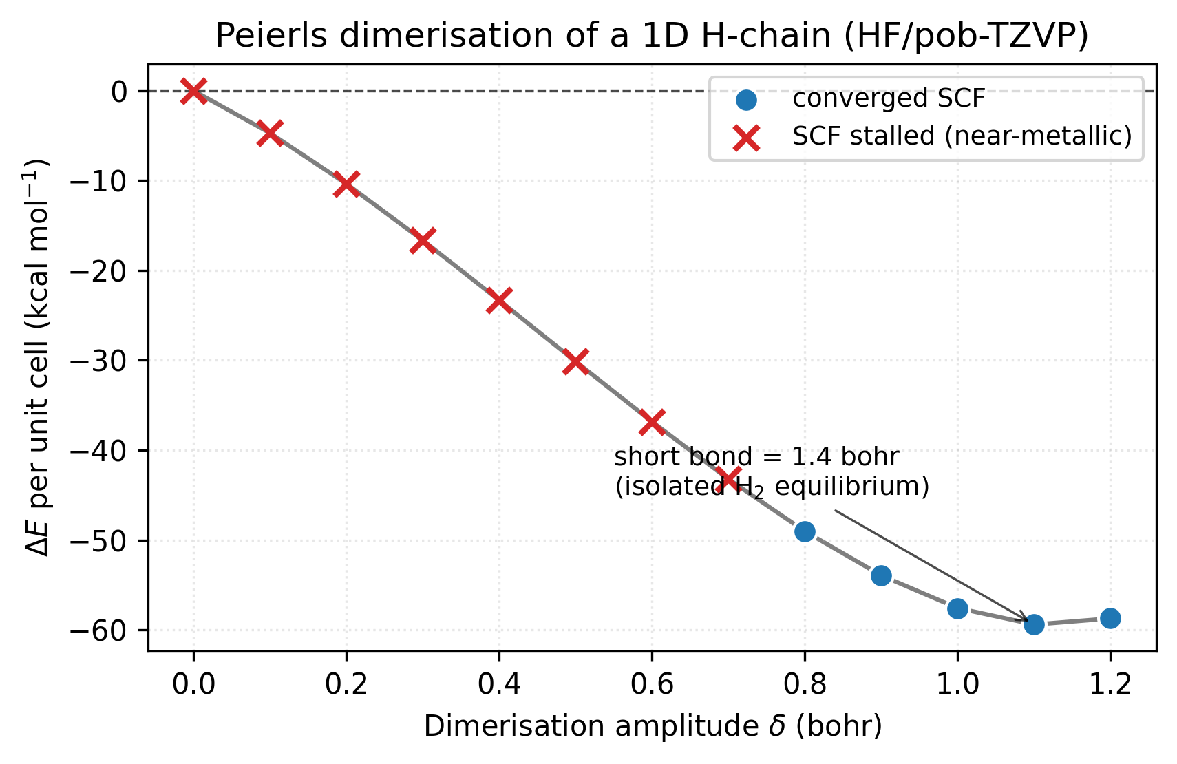
The energy drops by 62.6 kcal/mol per unit cell going from the uniform chain to the H₂-equilibrium dimerisation. All thirteen points of the finer scan converge on the k-point GDF route; a point whose SCF did not converge would be drawn as a red ✕. The minimum sits at \(\delta = 1.1\) bohr, short bond = 1.4 bohr = the isolated H₂ equilibrium, exactly as chemical intuition demands; at \(\delta = 1.2\) the energy rises again.

The energy curve is regenerated by [examples/plots/h-chain-peierls-energy.py](https://github.com/vibe-qc/vibe-qc/blob/main/examples/plots/h-chain-peierls-energy.py).

The dynamics of the dimerisation are clearer as an animation, the chain itself contracting at every other bond while the energy per cell falls:

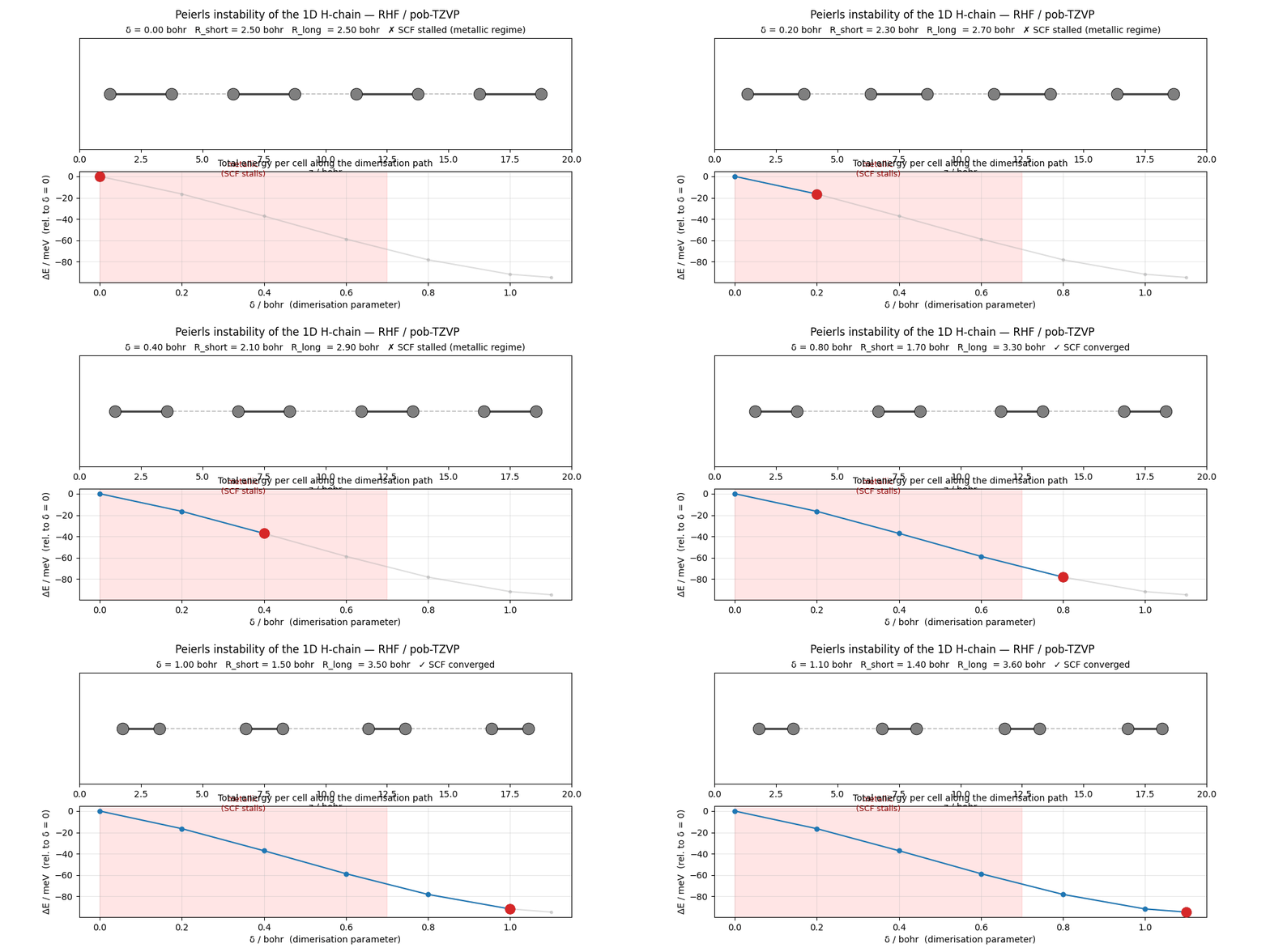
Regenerated by examples/plots/h-chain-peierls-animation.py. Two-panel layout: chain geometry on top (atoms moving toward their H₂-pair positions, bonds drawn solid for short / dashed for long), energy curve on the bottom (current δ marked, faint guide curve showing the rest of the path). The animation makes the mechanism of the instability immediate, it’s not just an abstract band crossing; it’s the lattice physically distorting to open the gap.

What the bands look like

Plot the bands at the two endpoints to see the gap-opening mechanism directly:

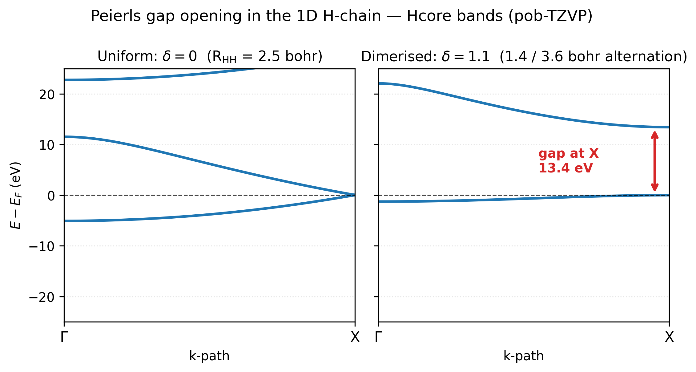
Left: the uniform chain (\(\delta = 0\)). With two H per cell at equal spacing the BZ is folded relative to the natural one-atom cell, so the two bands meet at the X point, that touch is the Peierls instability point, the place where the half-filled metallic band crosses \(E_F\). Right: the dimerised chain at \(\delta = 1.1\). The bands have separated cleanly: a deep, almost-flat bonding band sits below \(E_F\) (the localised H₂ σ orbital of every short bond), and a high antibonding band sits ~13 eV above (the σ*). The 13.4 eV gap at X is the Peierls gap, and it’s because this gap opens that the occupied bonding band drops, accounting for the energy stabilisation in the curve above.

The bands figure uses non-interacting (Hcore) bands, which is why the δ = 0 panel doesn’t depend on a converged SCF, Hcore needs none. Regenerated by [examples/plots/h-chain-peierls-bands.py](https://github.com/vibe-qc/vibe-qc/blob/main/examples/plots/h-chain-peierls-bands.py).

Caveat on the uniform end

The tolerance conv_tol_grad = 1e-3 is deliberately looser than the default. At small \(\delta\) the chain is near-metallic and the HF gradient can settle slowly while the energy has already stabilised to \(10^{-8}\); for the Peierls physics that is enough, because the relative energy across the scan is what matters. On the k-point GDF route every point of the seven-point scan converges in six or seven iterations, \(\delta = 0\) included, so the loose tolerance is a safeguard here rather than a necessity.

Theory

The sections below set out why the instability happens: the half-filled tight-binding band that makes the uniform chain metallic, the gap-opening period-doubling distortion that lowers its energy, why vibe-qc’s SCF reproduces the effect, and how the same argument extends to real materials.

The half-filled band

For the uniform chain with one H per unit cell, a tight-binding model with one orbital per site gives a single cosine band \(\varepsilon(k) = \varepsilon_0 - 2t \cos(ka)\), where \(t\) is the nearest-neighbor hopping. With one electron per site (half-filled), the Fermi level sits at \(k_F = \pi / 2a\), inside the band. The system is metallic.

The instability

Any perturbation of the lattice that opens a gap at \(\pm k_F\) lowers the occupied-state energy. The simplest perturbation with the right wavevector is a period doubling: atoms at \(\{\, 0, a, 2a, \dots \,\}\) redistribute to \(\{\, 0, a/2 + \delta_1, a, a + a/2 + \delta_2, \dots \,\}\) with alternating displacements. For a single-orbital tight-binding model, perturbation theory says the gain in band energy scales as \(\delta^2 \ln \delta\), while the elastic cost of distortion scales as \(\delta^2\). The logarithm wins at small \(\delta\), so the uniform chain is always unstable, for any non-zero electron- phonon coupling. This is the content of Peierls’ theorem (R. E. Peierls, Quantum Theory of Solids, Oxford University Press, 1955; see References).

In chemical language: the uniform chain is a delocalised half-filled band of s-orbitals. Dimerisation localises the electrons into bonding pairs in the short bonds, with empty antibonding in the long bonds, a classical valence-bond picture of alternating H₂ units with van-der-Waals spacers between.

Why vibe-qc sees this

Two-atom unit cells at the same spacing are crystallographically distinguishable from one-atom cells only by the basis you build, but the physics depends on the number of electrons per cell. A one-H-per-cell calculation is metallic; a two-H-per-cell calculation at \(\delta = 0\) has a one-band folded structure that should be metallic but is built in a basis set that doesn’t notice the symmetry equivalence. The restricted SCF still converges there on the 8-point mesh. That does not make the uniform chain an insulator: its folded bands touch at the zone boundary, and a closed-shell determinant on a finite mesh cannot represent the partially filled band, so read the uniform end of the scan with that in mind. As \(\delta\) grows the folded bands split, a real gap opens, and the energy drops.

Generalisation

The Peierls argument generalises far beyond the H-chain:

• Polyacetylene \((\text{CH})_n\), real 1D organic conductor, Peierls-distorted, bond alternation of about 0.08 Å (C=C about 1.36 Å, C-C about 1.44 Å) observed experimentally; the Su-Schrieffer-Heeger model (W. P. Su, J. R. Schrieffer and A. J. Heeger, Phys. Rev. Lett. 42, 1698 (1979), doi:10.1103/PhysRevLett.42.1698) is the tight-binding description of that distortion.

• Transition-metal dichalcogenide monolayers, 2D variants (charge-density waves) with more intricate wavevectors.

• 1D Jahn-Teller distortions in organic radicals.

Anywhere a regular lattice has a half-filled, partially-filled, or gapless band at a nesting vector \(\mathbf{Q}\), expect a distortion at wavevector \(\mathbf{Q}\) that opens a gap and lowers the energy.

Resources

About 12 minutes of wall time for the seven-point dimerisation scan at pob-TZVP / 8 k-points with 4 OpenMP threads, measured on a shared and heavily loaded laptop: each k-point GDF SCF takes 1.5 to 2 minutes. The cost grows with the transverse vacuum; for the RKS-PBE example of the same cell, one SCF took 26 s at 15 bohr against 64 s at 30 bohr, and the energy per cell moved by 3 µHa. If you push \(\delta \to 0\) further and the SCF struggles, level shifting helps.

References

• Original theorem. R. E. Peierls, Quantum Theory of Solids, Oxford University Press (1955), chapter 5. The textbook formulation and proof.

• Polyacetylene, original experiment. H. Shirakawa, E. J. Louis, A. G. MacDiarmid, C. K. Chiang, and A. J. Heeger, “Synthesis of electrically conducting organic polymers: halogen derivatives of polyacetylene, (CH)x,” J. Chem. Soc., Chem. Commun. 578 (1977), the experimental demonstration and one of the reasons they eventually won the 2000 Nobel Prize in Chemistry.

• SSH model, Peierls on polyacetylene. W. P. Su, J. R. Schrieffer, and A. J. Heeger, “Solitons in polyacetylene,” Phys. Rev. Lett. 42, 1698 (1979).

• Pseudopotential calculation on trigonal Te. J. D. Joannopoulos, M. Schlüter, and M. L. Cohen, “Electronic structure of trigonal and amorphous Se and Te,” Phys. Rev. B 11, 2186 (1975), empirical pseudopotential treatment of the crystalline phase, connecting the trigonal distortion to the observed band structure.

• Textbook, condensed-matter. G. Grüner, Density Waves in Solids, Addison-Wesley (1994), comprehensive modern treatment of Peierls-class instabilities in real materials.

Next

• Periodic geometry optimization could replace this manual scan. Periodic gradients and fixed-cell relaxation exist; see Periodic geometry optimization for which routes have analytic forces (Hartree-Fock relaxation falls back to finite-difference forces).

• For the intermediate, partially-metallic regime, Hubbard-\(U\)-corrected DFT and fractional-occupation smearing are the standard extensions. Both exist in vibe-qc, on the routes listed on those pages; check there before combining them with the GDF route used here.