The QVF file format, end to end

You will learn: what a .qvf archive is, the two ways vibe-qc produces one, the anatomy of its manifest, and how to write and read the main section-kind families, structure, scalar fields, the full wavefunction, spectra, electronic bands and density of states, optimisation and reaction paths, vibrations, and the provenance / citation metadata. By the end you will have produced three representative archives and validated them. The full current writer / viewer kind matrix lives in the QVF design doc; newer kinds such as basis.ao, scan.surface, COOP/COHP, Fermi surfaces, phonons, EOS, and QTAIM have dedicated examples or producer paths outside this compact showcase.

This is the format companion to vibe-view: an end-to-end walkthrough, which walks the vibe-view GUI. The vibe_view_walkthrough tutorial shows what a routine job emits; this tutorial shows the whole format surface and the lower-level writer API you reach for when you want to put something in a .qvf that run_job does not emit on its own.

Prerequisites:

• vibeqc installed and a working SCF setup (any Fundamentals tutorial).

• Optional: vibe-view installed (for the read-back and GUI steps), pip install -e 'vibe-view/[viewer]' from the checkout root.

Time to complete: about 15 minutes.

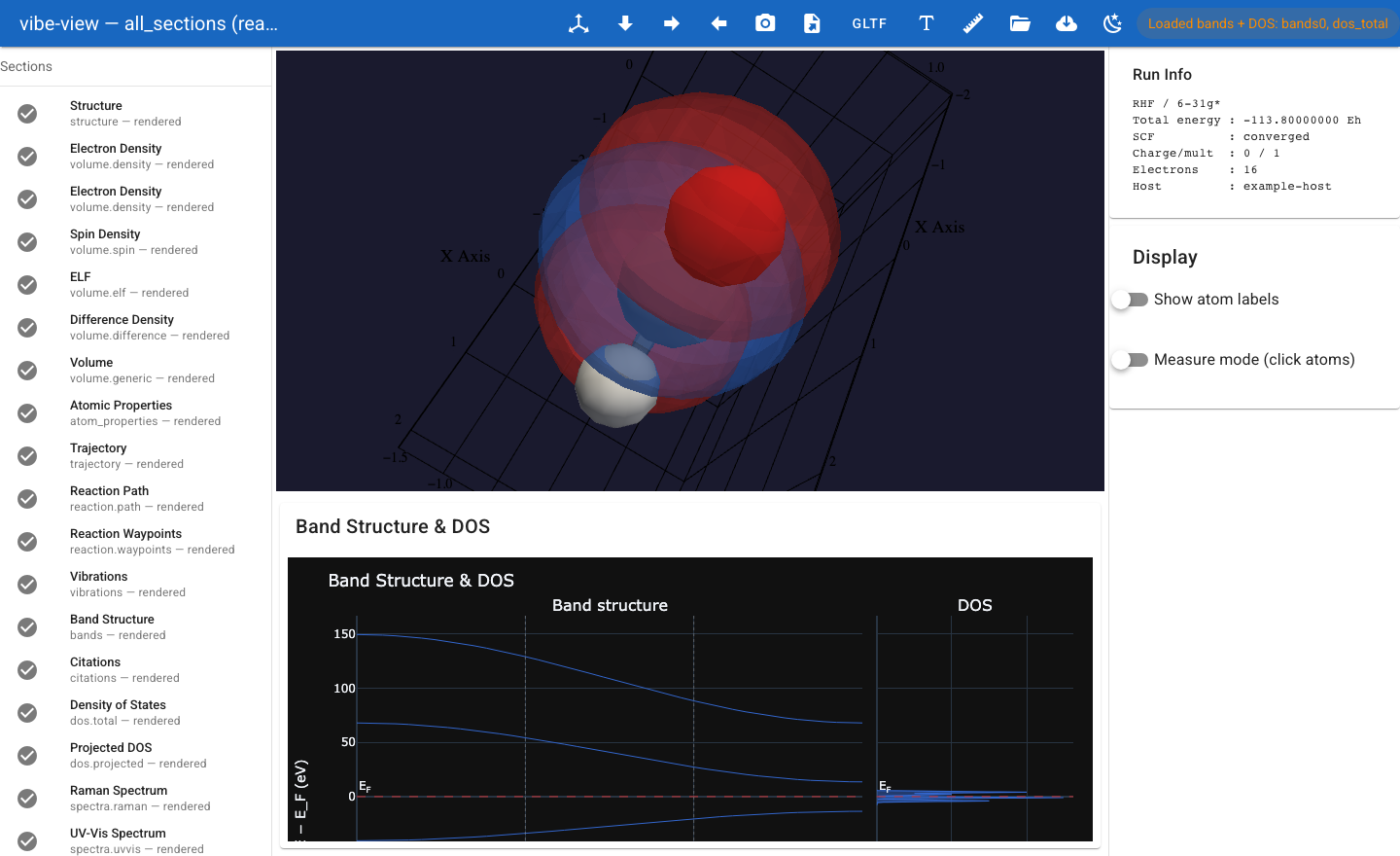
One QVF archive opened in vibe-view — a bands + dos.total figure on a shared energy axis. By the end of this tutorial you will have written and validated a representative multi-section .qvf bundle.

1. What a .qvf is

A .qvf (Quantum Visualization Format) is a single ZIP archive that bundles everything a calculation produced for visualization, geometry, scalar fields, spectra, bands, trajectories, provenance, instead of scattering it across .cube, .xyz, .molden, .xsf and log files. One file you can hand to a colleague, attach to a paper’s SI, or open in vibe-view.

Inside, it is just a ZIP with three layers:

water.qvf
├── manifest.json              # the index: every section + member, with checksums
├── structure/structure.json   # JSON members (small, human-readable)
├── volumes/density.dat         # binary members (large numeric arrays)
├── volumes/density_grid.json
├── ...

• manifest.json is the single source of truth. It lists every section (a unit of content like “the electron density” or “the IR spectrum”), and within each section the members (the files that carry the bytes), each with a path, a format (json or binary), and a sha256 checksum.

• JSON members carry small structured data (atom lists, spectrum peaks, grid descriptors).

• Binary members carry large numeric arrays (volumetric grids, MO coefficients, trajectory coordinates) as raw little-endian buffers, with their dtype and shape declared in the manifest.

The canonical contract is the JSON Schema at python/vibeqc/output/formats/qvf_manifest.schema.json; the full specification (units, section kinds, the validation and extension models) is the QVF design doc.

The write-time validation gate

write_qvf validates the archive it just wrote against the canonical schema before returning, and if validation fails it deletes the file and raises. A .qvf on disk that came from vibe-qc is therefore guaranteed schema-valid. This is also why the showcase script in this tutorial is a useful bug-finder: writing one archive per section kind and getting no exception is the test that every writer path is sound.

2. Two ways to produce a .qvf

There are two routes to an archive: the high-level output_qvf=True flag on a normal job, which covers almost every case, and the lower-level write_qvf(...) call for sections a job does not emit on its own.

a. The natural way, output_qvf=True

Any run_job / run_periodic_job call emits a .qvf when you pass output_qvf=True. The sections that appear are whatever the job computed: ask for cubes and you get volume.*; ask for a Hessian and you get vibrations + spectra.ir; optimise and you get a trajectory. This is what vibe-view: an end-to-end walkthrough uses, and it is what you want 95% of the time:

from vibeqc import Atom, Molecule, run_job

mol = Molecule([
    Atom(8, [0.0,  0.00,  0.00]),
    Atom(1, [0.0,  1.43, -0.98]),
    Atom(1, [0.0, -1.43, -0.98]),
])

run_job(
    mol, basis="6-31g*", method="rhf",
    optimize=True,                 # -> trajectory
    hessian=True,                  # -> vibrations + spectra.ir
    write_cube=["density", "homo", "lumo"],  # -> volume.density + volume.orbital
    write_molden_file=True,        # -> wavefunction.gto
    write_population_file=True,    # -> atom_properties
    citations=True,                # -> citations
    output="water", output_qvf=True,
)

b. The explicit way, write_qvf(...)

To put something in a .qvf that run_job does not emit, a difference density you computed yourself, a UV/Vis spectrum from an external tool, hand-built reaction-path waypoints, call the writer directly. It takes an OutputPlan and a bag of context keyword arguments, one per section kind:

from vibeqc.output.formats.qvf import write_qvf, validate_qvf
from vibeqc.output.plan import OutputPlan

plan = OutputPlan.from_run_job_kwargs(
    output="custom", method="rhf", basis="sto-3g", functional=None
)

write_qvf(
    "custom", plan,
    molecule=mol,                              # -> structure
    volume_data={"Density": (rho, origin, span)},  # -> volume.density
    raman_data={"frequencies": [...], "intensities": [...]},  # -> spectra.raman
    # ... one kwarg per section you want ...
)

The rest of this tutorial walks the representative section families and the context keys that produce them. The full runnable compact showcase is examples/vibe_view/showcase_qvf_all_sections.py, it builds three archives covering the historical 27-kind gate and validates each. Run it now and refer back to its output as you read:

~/path/to/vibeqc/.venv/bin/python examples/vibe_view/showcase_qvf_all_sections.py

3. Anatomy of the manifest

Open any archive and read its manifest, this is the consumer’s entry point:

import zipfile, json
manifest = json.loads(zipfile.ZipFile("water.qvf").read("manifest.json"))

print("QVF v", manifest["qvf_version"])
print("from ", manifest["source"])           # program, version, calculation
print("provenance", manifest.get("provenance"))  # method, basis, energy, ...
for s in manifest["sections"]:
    print(f"  {s['id']:<16s} {s['kind']}")

The manifest root carries:

• qvf_version, always 1, including for periodic reaction paths, whose per-frame lattices ride as an optional member (see § 8).

• source, producer program, version, and a calculation string.

• provenance, best-effort method / functional / basis / charge / multiplicity / SCF energy / convergence (assembled from the context you pass).

• viewer_defaults, optional producer hints (which section to auto-open, default isovalue / colormap, camera bookmarks).

• sections, the list. Each entry has an id, a kind, optional label, and a members map of role → member spec. A member spec is {path, format, sha256} for JSON and additionally {dtype, shape} for binary.

All units follow the format’s conventions (positions in Å, grids in bohr, energies in Hartree or eV per the units table).

4. The section kinds, group by group

Every snippet below is a context kwarg to write_qvf. The showcase script assembles them into coherent archives; here they are isolated so you can see exactly what each kind needs.

4.1 Structure and connectivity

The structure kind carries the geometry, with optional bonds and structure.symmetry members alongside it:

write_qvf(
    stem, plan,
    molecule=mol,                       # structure  (or system=PeriodicSystem)
    bonds_data=[(0, 1, 1.0), (0, 2, 1.0)],   # bonds — (i, j, order) triples
    symmetry_data={                     # structure.symmetry  (spglib-style)
        "space_group_number": 225,
        "space_group_symbol": "Fm-3m",
        "point_group": "m-3m",
    },
)

structure is the one section almost every archive has. Pass molecule= for a molecule or system= for a PeriodicSystem (which adds lattice vectors and pbc flags). bonds is an explicit connectivity table (omit it and the viewer infers bonds from covalent radii); structure.symmetry carries the spglib summary.

4.2 Scalar fields, the six volume.* kinds

All volumes share the same shape: a dict {label: (data_3d, origin, span)} where data_3d is a 3-D numpy array, origin is the grid anchor in bohr, and span is the 3×3 matrix of per-voxel step vectors in bohr.

write_qvf(
    stem, plan, molecule=mol,
    volume_data={"Electron density": (rho, origin, span)},   # volume.density
    mo_data=[...],                                           # volume.orbital
    spin_data={"Spin density": (s, origin, span)},           # volume.spin
    elf_data={"ELF": (elf, origin, span)},                   # volume.elf
    generic_volume_data={"RDG": (rdg, origin, span)},        # volume.generic
    diff_data={"Δρ": {                                       # volume.difference
        "data": diff, "origin": origin, "span": span,
        "operand_a": "vol_dens_0", "operand_b": "vol_dens_0",
        "description": "ρ(product) − ρ(reactant)",
    }},
)

• volume.density / volume.spin / volume.elf differ only in meaning and the viewer’s default colormap (signed for spin and difference, sequential for density and ELF).

• volume.generic is the escape hatch for any scalar field that is not one of the named kinds (reduced density gradient, electrostatic potential you computed yourself, …).

• volume.difference can link to the two volume.* sections it was built from via operand_a / operand_b (section ids), so a viewer can offer “show me the operands”.

• mo_data (the volume.orbital kind) is a list of per-orbital dicts; the qvf_mo_data(result, basis, molecule, indices) helper builds it for you from a finished SCF (pass the orbital indices to sample), and run_job(write_cube=[...]) produces it automatically.

For the full molecular orbital set without pre-sampling every orbital, use the wavefunction section instead (next).

4.3 The wavefunction, wavefunction.gto

The wavefunction.gto kind stores the full GTO basis and MO coefficients so a viewer can resample any orbital on demand; the qvf_wf_data helper builds it from a finished SCF:

from vibeqc.output.formats.qvf import qvf_wf_data
write_qvf(stem, plan, molecule=mol,
          wf_data=qvf_wf_data(result, basis, mol))   # wavefunction.gto

This embeds the GTO basis (shells, exponents, contraction coefficients) plus the MO coefficient matrix, so a viewer can resample any orbital on demand, far cheaper than writing each orbital as its own volume.orbital. run_job(write_molden_file=True) emits it automatically. Unrestricted runs carry separate α/β coefficient members.

Shell coefficients in the archive apply to normalized primitive Gaussians (see docs/design_qvf_format.md § 4.6 for the formula). The writer handles this automatically, you pass raw libint shells and qvf_wf_data does the conversion.

4.4 The spectra family, seven kinds

Each spectrum is a small JSON dict of peaks. They share a common {frequencies, intensities} core; the energy-axis kinds accept energies_ev and the writer maps it for you.

write_qvf(
    stem, plan, molecule=mol,
    # spectra.ir is emitted automatically from a Hessian (hessian_result=)
    raman_data={"frequencies": fr, "intensities": ri},          # spectra.raman
    uvvis_data={"energies_ev": e, "intensities": f},            # spectra.uvvis
    ecd_data={"energies_ev": e, "intensities": R},              # spectra.ecd
    vcd_data={"frequencies_cm1": fr, "intensities": dA},        # spectra.vcd
    nmr_data={"isotope": "1H", "chemical_shifts": [...]},       # spectra.nmr
    generic_spectrum_data={                                     # spectra.generic
        "section_id": "xps", "label": "XPS",
        "frequencies": [...], "intensities": [...],
    },
)

spectra.ir is special: it is derived from a HessianResult (pass hessian_result=, or use run_job(hessian=True)), not a hand-built dict, the writer computes the intensities. The other six accept producer-supplied numbers, which is what you want when the spectrum came from a method vibe-qc does not yet compute. spectra.generic lets you name your own axis for anything that does not fit (XPS, a fitted envelope, …).

Warning

The synthetic spectra in the showcase script are illustrative format-demo data, not computed observables. The format supports carrying these spectra; vibe-qc does not yet compute most of them. Do not cite numbers read out of a demo archive.

4.5 Electronic structure of solids, bands, dos.total, dos.projected

The periodic-only kinds carry a band structure along a k-path plus total and projected densities of states; they need system= rather than molecule=:

write_qvf(
    stem, plan, system=periodic_system,
    band_structure=vq.band_structure_hcore(sys, basis, kpath),   # bands
    dos_data={                                                   # dos.total
        "energies": E, "dos": g, "n_spin": 1,
        "smearing": 0.1, "fermi_energy_ev": 0.0, "n_electrons": 20.0,
    },
    pdos_data={                                                  # dos.projected
        "energies": E, "projections": g_channels, "n_spin": 1,
        "channels": [{"atom_index": 1, "symbol": "O", "l": 1, "label": "O 2p"}],
    },
)

bands takes a real BandStructure (the cheapest is band_structure_hcore, which needs no SCF, see Band structure and density of states). DOS arrays are [n_points] (or [2, n_points] for spin-polarized total DOS, [n_channels, n_points] for projected); energies are in eV with the Fermi level at 0. These are the periodic-only kinds, they need system= rather than molecule=.

Validated periodic chi-CCM-B QVF fixtures

The documentation tree also carries two small periodic QVF fixtures from jk_method="aiccm2026dev-b" that exercise the finite-BvK torus path in vibe-view. They are useful when checking a consumer’s periodic box, grid, replication, and vendor-overlay behavior because they contain only precomputed periodic volume.density / volume.orbital grids, not a periodic wavefunction.gto section.

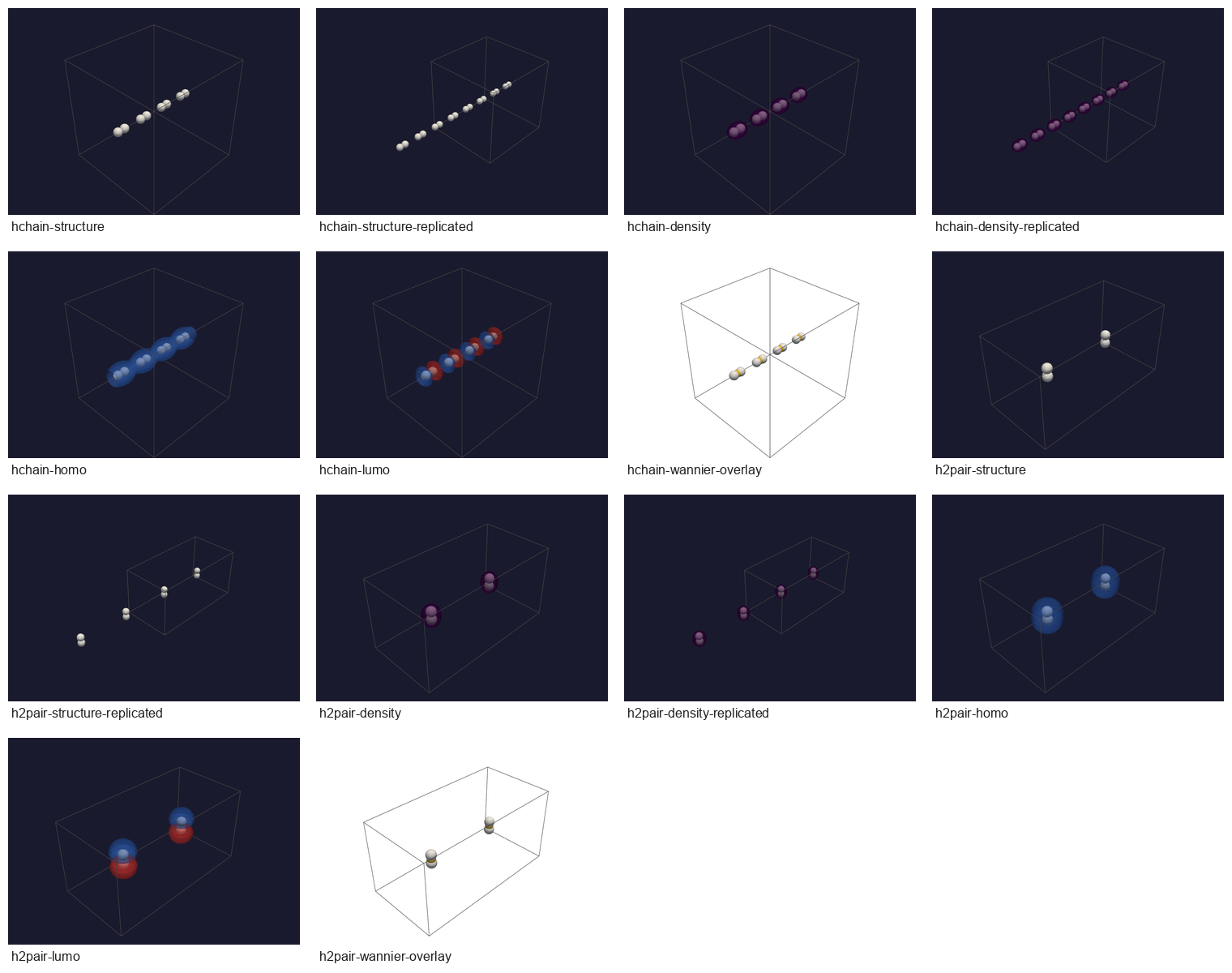
Headless vibe-view captures for the two chi-CCM-B periodic QVF fixtures: single-cell and replicated structures, density surfaces, orbital surfaces, and x_ccm.wannier_centers overlays.

Case	Input	Full output	System manifest	QVF archive	Captures
3D vacuum-padded H-chain, RI, aiccm_lattice_extension=(4,1,1)	input	.out	.system	.qvf	structure, replicated structure, density, replicated density, HOMO, LUMO, Wannier overlay
3D H2-pair, RI, aiccm_lattice_extension=(2,1,1)	input	.out	.system	.qvf	structure, replicated structure, density, replicated density, HOMO, LUMO, Wannier overlay

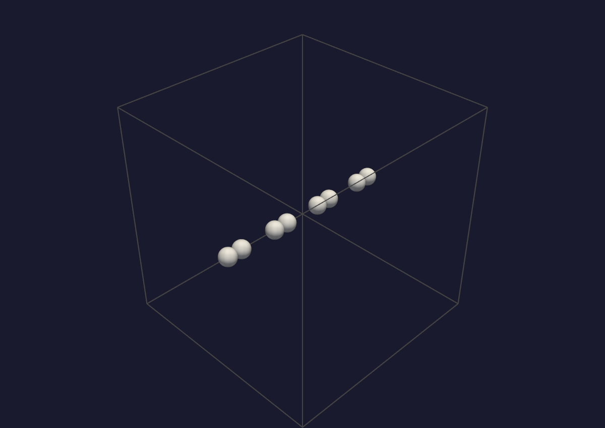
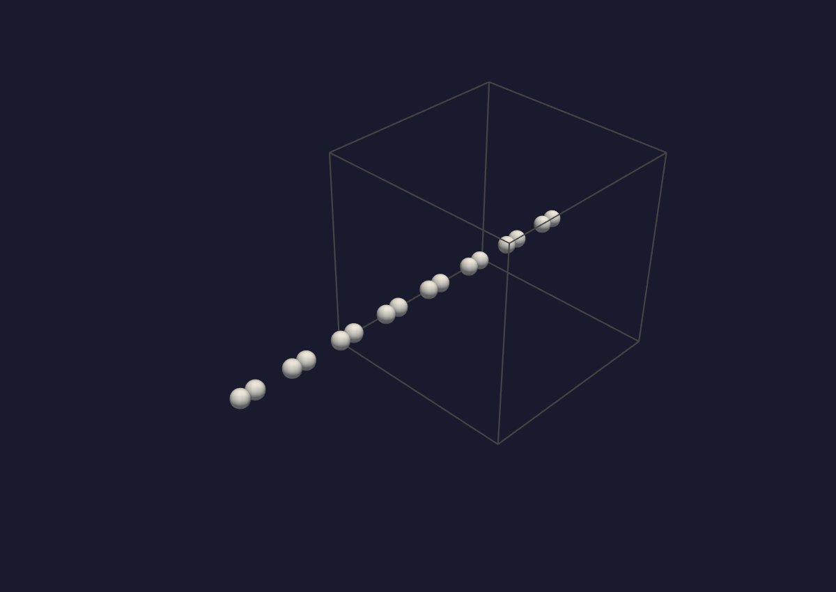
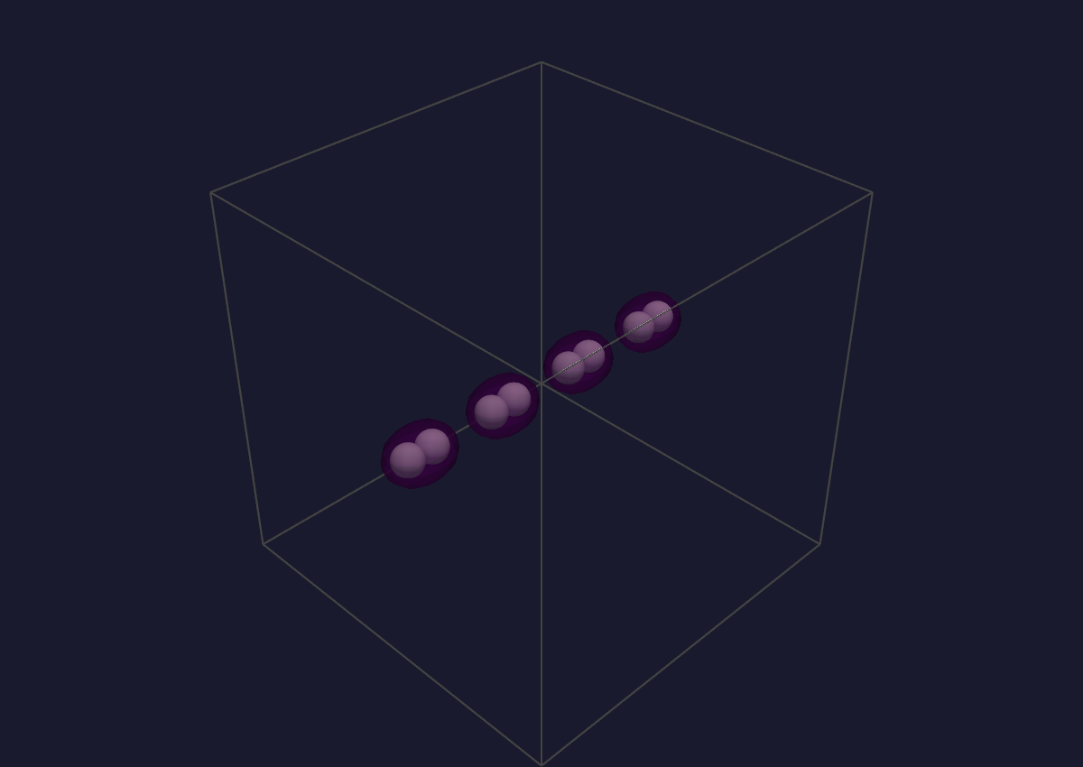
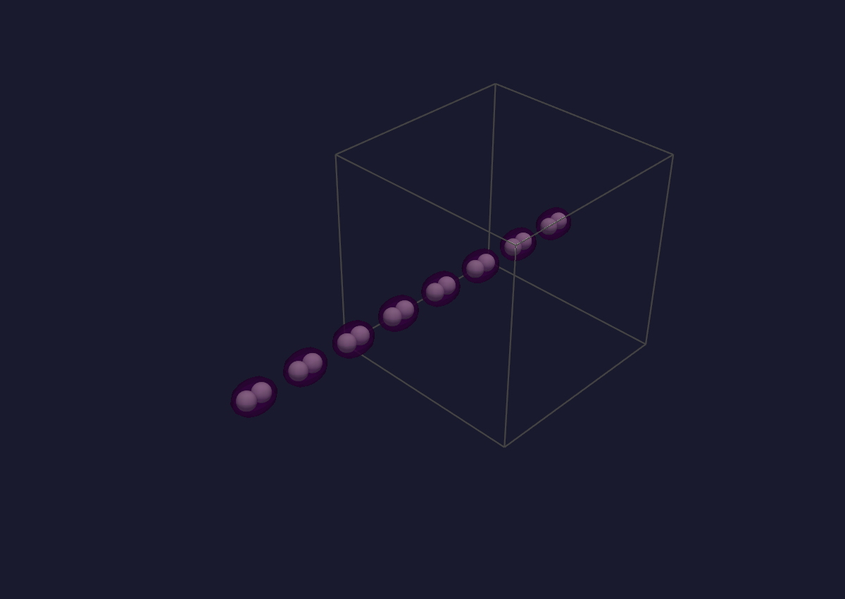
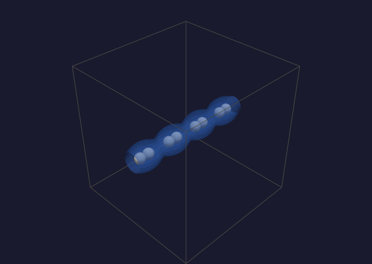
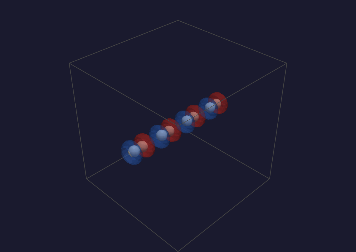
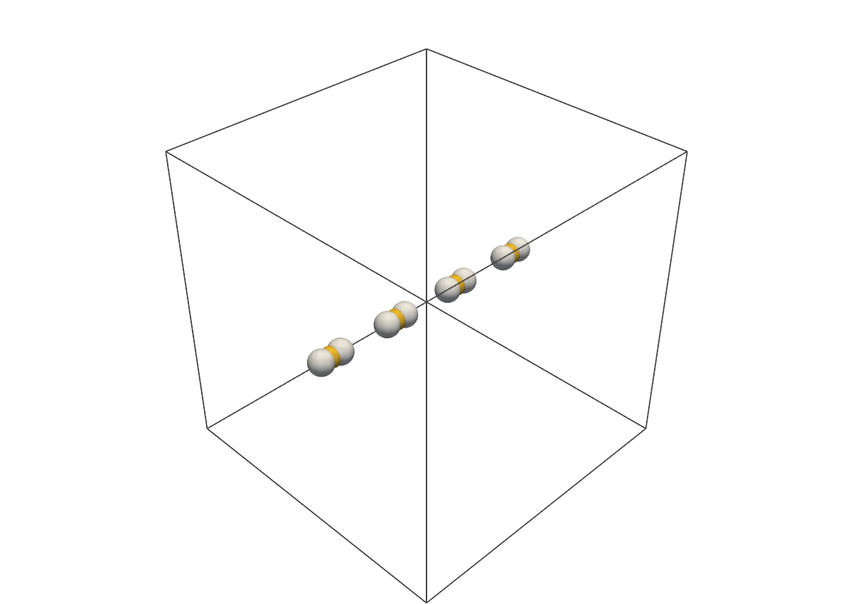
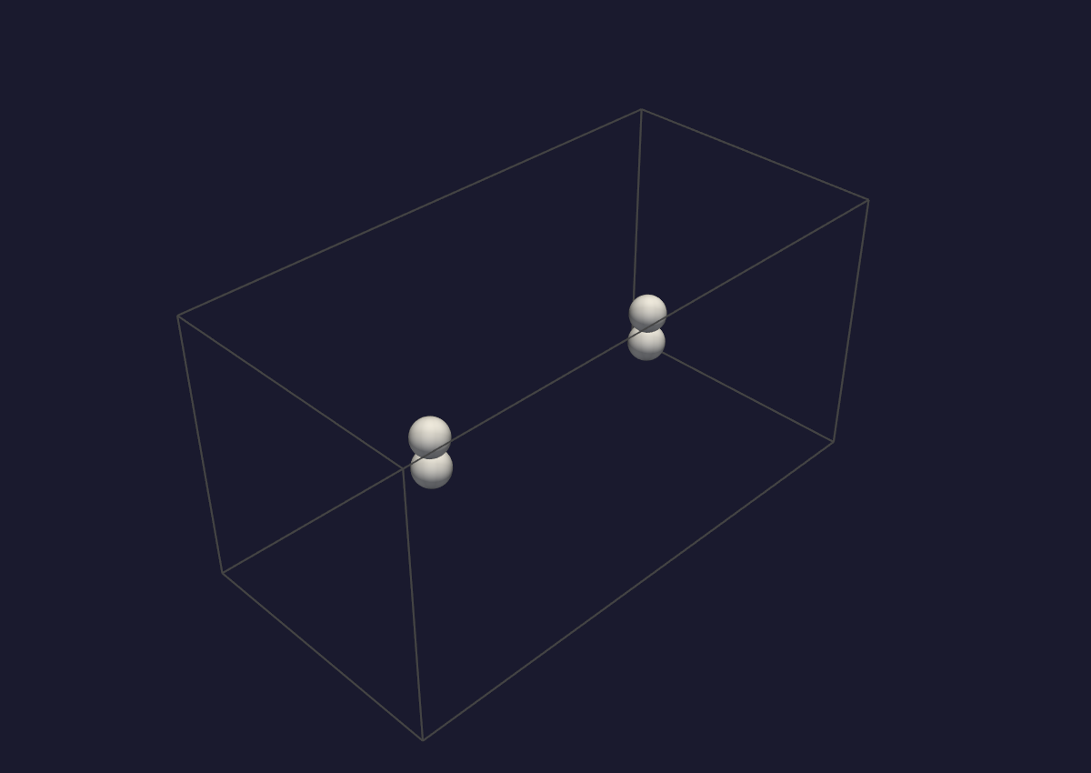
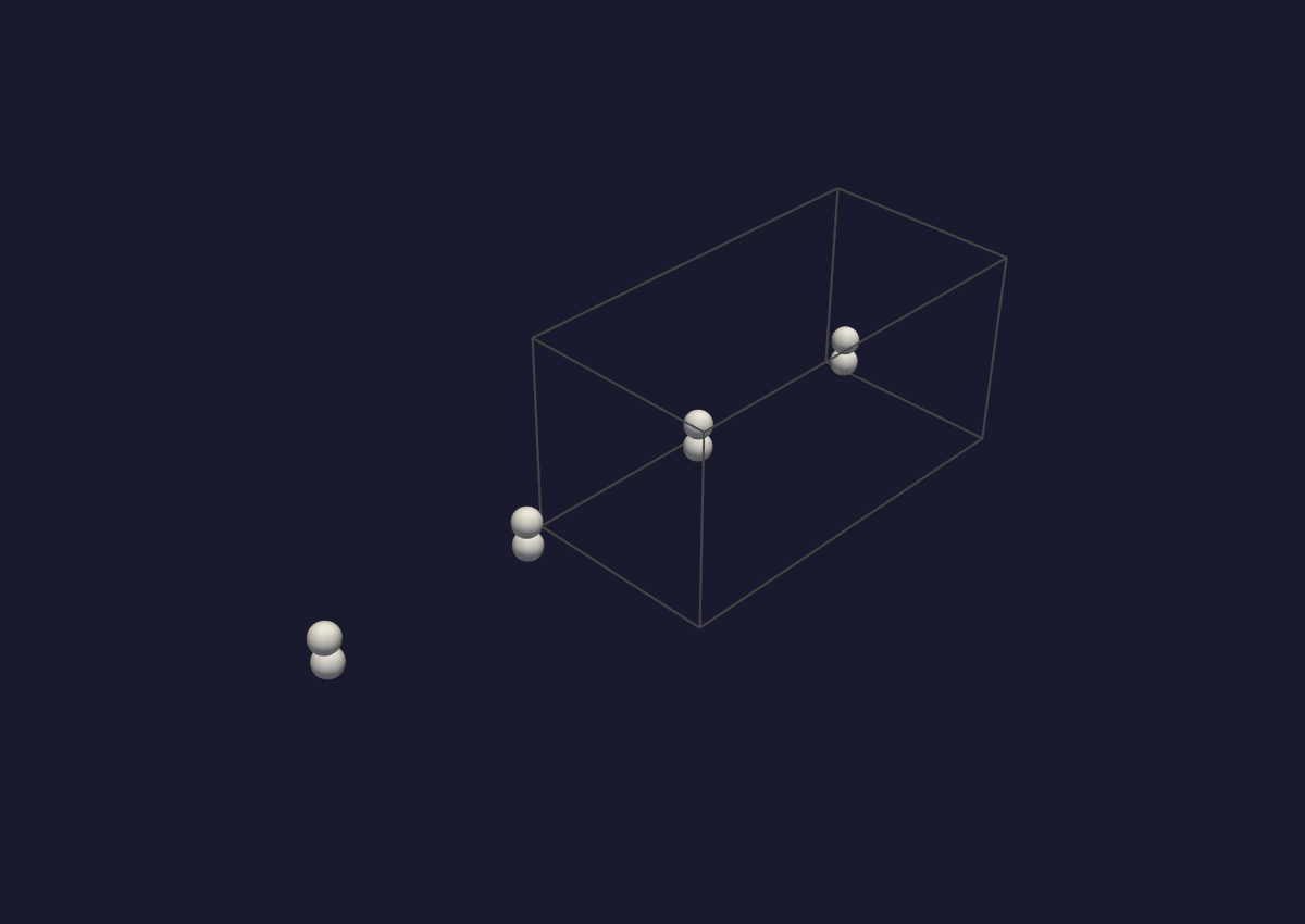
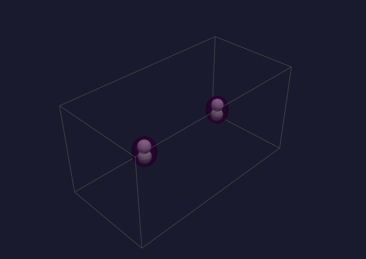
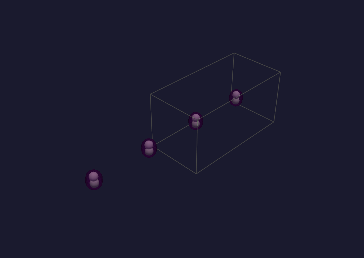
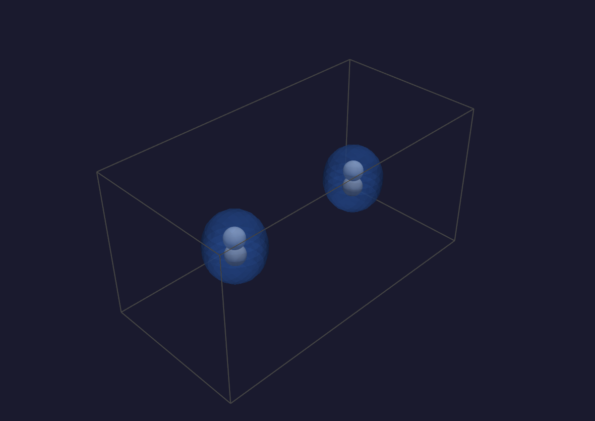
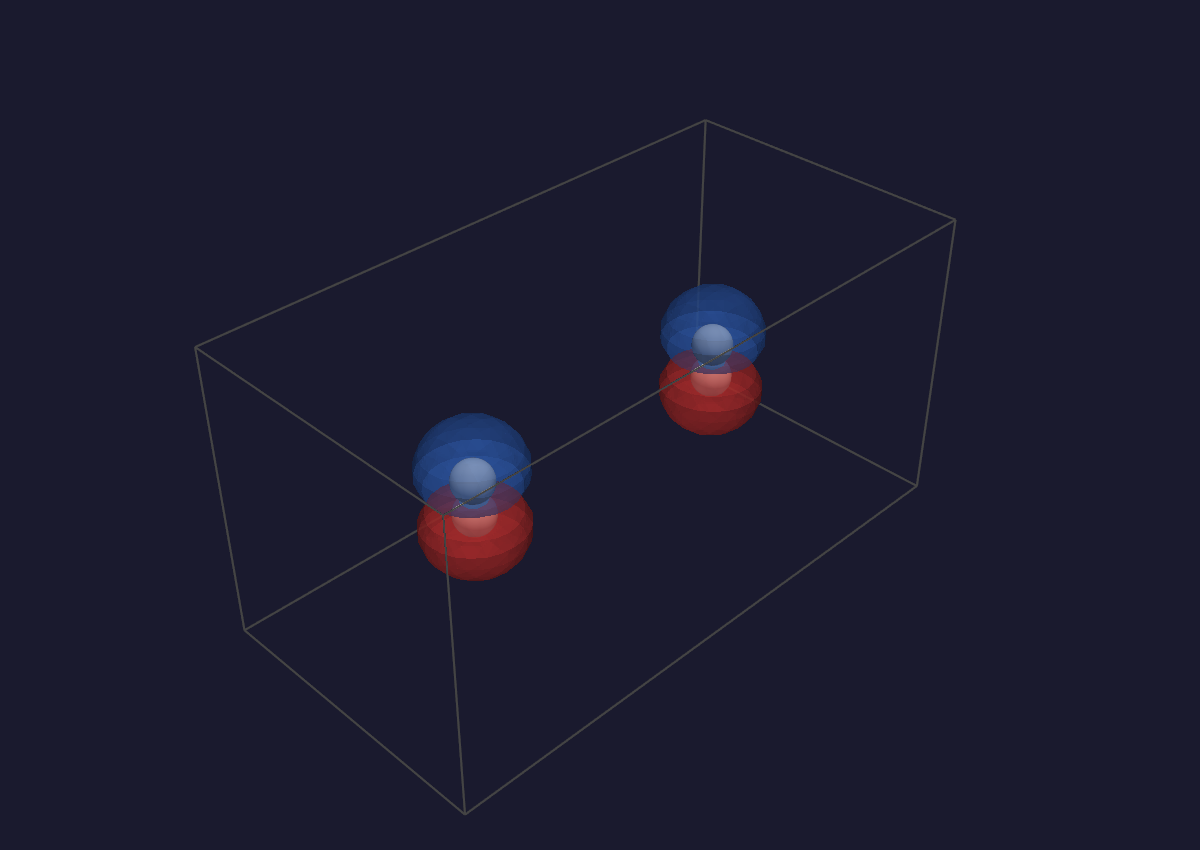
The vacuum-padded H-chain archive has structure.pbc=[true,true,true], structure.dimensionality=3, a 40 x 40 x 40 density grid spanning the full 20 x 20 x 20 bohr BvK supercell, and integrates to 8.001083 electrons. The H2-pair archive has structure.pbc=[true,true,true], structure.dimensionality=3, a 48 x 24 x 24 grid spanning 24 x 12 x 12 bohr, and integrates to 4.000538 electrons. Both archives validated with validate_qvf(...) after the public copies were sanitized.

4.6 Paths and dynamics, trajectory, reaction.path, reaction.waypoints, vibrations

These kinds carry a stack of geometries (an optimisation or MD run), a typed reaction path or its lightweight waypoint annotation, and normal-mode displacements from a Hessian:

write_qvf(
    stem, plan, molecule=mol,
    trajectory_frames=frames,            # trajectory  (list of Molecule)
    trajectory_energies=[...],
    reaction_waypoints={                 # reaction.waypoints (annotates traj0)
        "trajectory_ref": "traj0",
        "waypoints": [{"frame_index": 0, "label": "start", "kind": "point"}],
    },
    reaction_path={                      # reaction.path (self-contained)
        "frames": rxn_frames,
        "energies": [...],
        "waypoints": [
            {"frame_index": 0, "label": "Reactant", "kind": "reactant"},
            {"frame_index": 2, "label": "TS", "kind": "transition_state"},
            {"frame_index": 4, "label": "Product", "kind": "product"},
        ],
    },
    hessian_result=hess,                 # vibrations  (+ spectra.ir)
)

• trajectory is a stack of geometries (a geometry optimisation, an MD run), frames are Molecule objects, optionally with per-frame energies. run_job(optimize=True) emits one.

• reaction.path is a self-contained path with typed waypoints (reactant / transition_state / intermediate / product / point), exactly what an NEB run produces.

• reaction.waypoints is the lightweight alternative: instead of re-storing coordinates, it annotates a trajectory already in the archive (the trajectory_ref must name a trajectory section in the same file, or the writer raises).

• vibrations carries normal-mode displacements from a HessianResult; passing one also emits spectra.ir.

4.7 Provenance and metadata, atom_properties, scf_history, citations, viewer_defaults

The metadata kinds carry per-atom charges, the per-iteration SCF history, the embedded BibTeX bundle, and the manifest-root viewer hints:

write_qvf(
    stem, plan, molecule=mol,
    population_summary=pop,               # atom_properties (Mulliken/Löwdin)
    scf_history_data=[                    # scf_history
        {"iter": 0, "energy_eh": -74.9, "delta_e": 1.0, "diis_error": 0.5},
    ],
    bibtex_content=open("water.bibtex").read(),   # citations
    viewer_defaults={                     # manifest-root hints
        "auto_open": ["vol_dens_0"],
        "vol_dens_0": {"isovalue": 0.05, "colormap": "viridis"},
    },
)

atom_properties carries per-atom Mulliken / Löwdin charges; scf_history the per-iteration energy and DIIS error; citations the embedded BibTeX bundle (the same bytes as the .bibtex sidecar, see Auto-citations: from .out to manuscript bibliography). viewer_defaults is not a section but a manifest-root block of hints the viewer honours on load.

5. Run the showcase, three representative archives

The script produces:

Archive	Built by	Kinds it contributes
water.qvf	real run_job	structure, volume.density, volume.orbital, wavefunction.gto, trajectory, vibrations, spectra.ir, atom_properties, scf_history, citations
spectroscopy.qvf	explicit write_qvf	volume.spin / elf / difference / generic, spectra.raman / uvvis / ecd / vcd / nmr / generic, structure.symmetry, bonds, reaction.path, reaction.waypoints, viewer_defaults
crystal.qvf	explicit write_qvf	bands, dos.total, dos.projected, periodic structure, structure.symmetry, periodic reaction.path

The final lines of its output are the coverage gate:

Coverage gate:
  kinds covered: 27/29
...
 All 27 implemented section kinds written, validated, and round-tripped (basis.ao + scan.surface exercised separately).

The numbers above are the historical compact-showcase gate for those three archives, not the full current QVF registry. If one of those writer paths regresses, the script dies at the offending write_qvf call (the validation gate) or at the coverage assertion, which is exactly the bug-finding behaviour we want from it.

6. Validate and read back

You do not need vibe-view to consume a .qvf, it is a documented ZIP. The producer-side gate already validated it, but you can re-check:

from vibeqc.output.formats.qvf import validate_qvf
report = validate_qvf("crystal.qvf")
assert report["valid"], report["errors"]

To read it with nothing but the standard library, verifying checksums yourself, then pulling a binary array out, follow the QVF consumer reference. The essential move for a binary member is np.frombuffer(zf.read(m["path"]), dtype=m["dtype"]).reshape(m["shape"]). The showcase script’s _verify_one_checksum does the SHA-256 round-trip in a few lines.

If vibe-view is installed, its reader gives you the same manifest plus classification of which kinds it can render:

from vibeview.qvf import QVFReader
reader = QVFReader("spectroscopy.qvf")
print(len(reader.manifest["sections"]), "sections")

7. Open it in vibe-view

If vibe-view is installed, point it at one of the archives to browse every section you wrote, panel by panel:

vibe-view open examples/vibe_view/runs/qvf_showcase/spectroscopy.qvf

The startup banner lists every section as rendered / skipped, and the browser opens at http://127.0.0.1:8080. Walk the sidebar, each kind this tutorial wrote has its own panel.

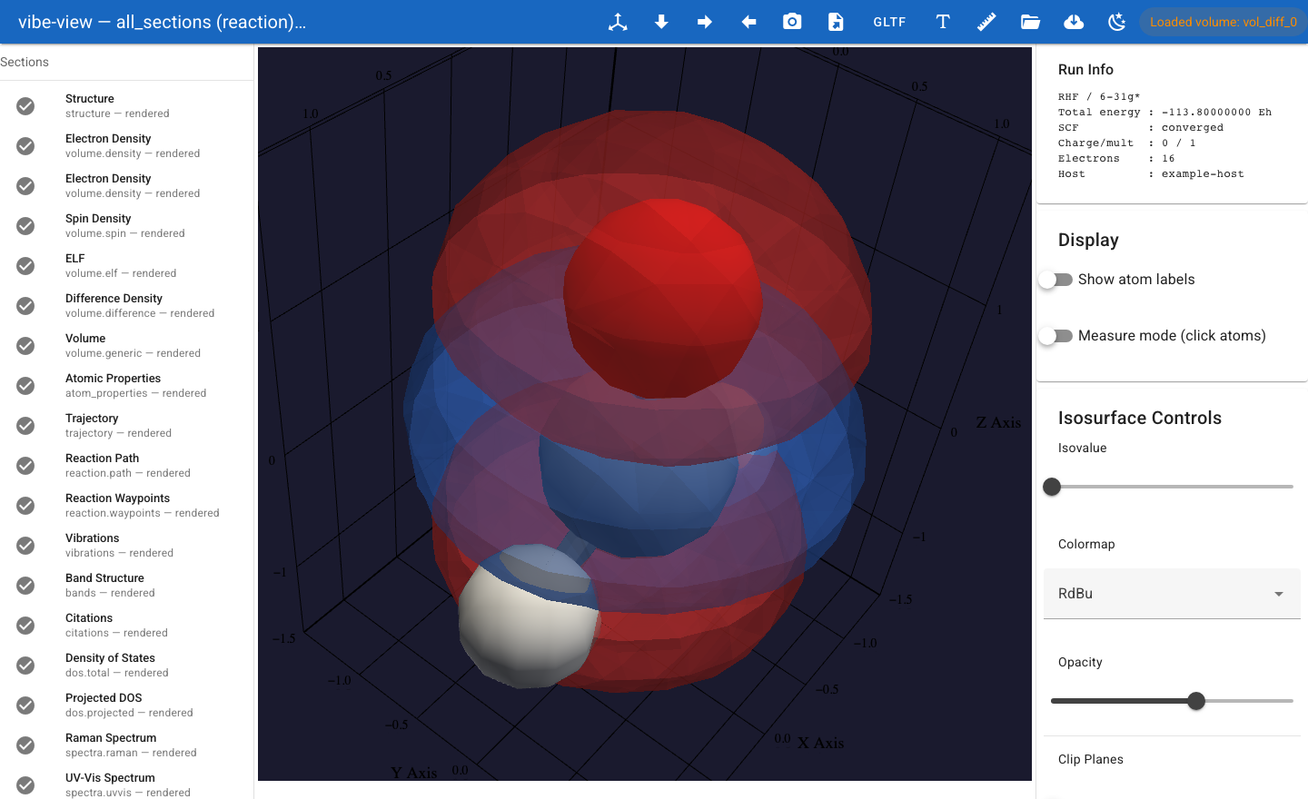
A two-colour difference-density isosurface (blue = positive, red = negative) — one of the panels spectroscopy.qvf opens with.

See vibe-view: an end-to-end walkthrough for the panel-by-panel tour and the vibe-view user guide for every control.

8. Versioning, reserved kinds, and extensions

• v1 vs v2. Current producers emit qvf_version=1. Periodic reaction.path and trajectory sections may carry optional per-frame lattice vectors and dimensionality metadata, but those are additive v1 fields. The earlier qvf_version=2 bump for periodic paths was withdrawn: consumers should still accept old archives labelled qvf_version=2 as v1-compatible, but new producers should not emit that label.

• Reserved kinds. Portable canonical kinds live in the design-doc registry. If you need experimental data before a kind is promoted there, use volume.generic, spectra.generic, or a vendor namespace such as x_<vendor>.* instead of inventing an unregistered canonical name.

• Vendor extensions. A producer can write its own section under the x_<vendor>.* namespace. Consumers that do not understand it skip it (“skipped, vendor namespace”) rather than refusing the file, unless the section is flagged critical. The extension model is the governance for promoting a vendor kind to a canonical one.

Next

• vibe-view walkthrough, the GUI tour of these sections.

• QVF design doc, the full format specification: units, every section schema, the validation and extension models.

• QVF consumer reference, read .qvf files programmatically without the viewer.

• auto citations, how the citations section is assembled.

• NEB reaction paths, the natural source of reaction.path sections.