Band structure and density of states
This tutorial uses a one-dimensional H2 chain to teach k paths, k meshes, band arrays, Gaussian broadening, and DOS normalization. It deliberately uses the non-self-consistent Hcore operator so the exercise is fast.
Important
Hcore contains kinetic and nuclear-attraction terms only. The plot produced here is a teaching model, not an HF or DFT prediction for a hydrogen crystal. For a scientific band, DOS, or PDOS claim, use a route-specific helper that diagonalizes the converged SCF operator and verify that exact operator in the calculation record.
For the equations, route-specific SCF helpers, and interpretation checklist, see Band structure and DOS.
Build and sample the chain
The unit cell contains one H2 molecule. The real periodic direction is x; the other lattice columns are bookkeeping separation for this 1D example.
The band path and DOS mesh are intentionally different:
the path follows \(\Gamma\rightarrow X\) to show dispersion;
the mesh samples the full 1D Brillouin zone to integrate the DOS.
import numpy as np
import vibeqc as vq
from vibeqc.plot import bands_dos_figure

system = vq.PeriodicSystem(
    dim=1,
    lattice=[[6.0, 0.0, 0.0], [0.0, 30.0, 0.0], [0.0, 0.0, 30.0]],
    unit_cell=[
        vq.Atom(1, [0.0, 0.0, 0.0]),
        vq.Atom(1, [1.4, 0.0, 0.0]),
    ],
)
basis = vq.BasisSet(system.unit_cell_molecule(), "sto-3g")

kpath = vq.kpath_from_segments(
    system,
    [((0.0, 0.0, 0.0), "Γ", (0.5, 0.0, 0.0), "X")],
    points_per_segment=40,
)
bands = vq.band_structure_hcore(
    system,
    basis,
    kpath,
    n_electrons_per_cell=2,
)
dos = vq.density_of_states_hcore(
    system,
    basis,
    mesh=[80, 1, 1],
    sigma=0.02,
    n_electrons_per_cell=2,
)

print("band array:", bands.energies.shape)
print("Gamma energies:", bands.energies[0])
print("X energies:", bands.energies[-1])
print("occupied reference:", bands.e_fermi)

dos_area = np.trapezoid(dos.dos, dos.energies)
print(f"integrated DOS: {dos_area:.6f}; expected {basis.nbasis}")

fig = bands_dos_figure(bands, dos, title="H2 chain (STO-3G, Hcore)")
fig.savefig("h-chain-hcore-bands-dos.png", dpi=180)
STO-3G supplies one AO per hydrogen, so the two-atom unit cell produces two
bands. points_per_segment=40 means 40 intervals including both endpoints, so
this one-segment path has 41 points and bands.energies has shape (41, 2).
For a multi-segment path, the builder counts a shared endpoint only once.
The DOS integral should be close to two because each unit-area Gaussian represents one band state after normalized k-point weighting. A value below two usually means the energy grid cuts off Gaussian tails.
Read the plot
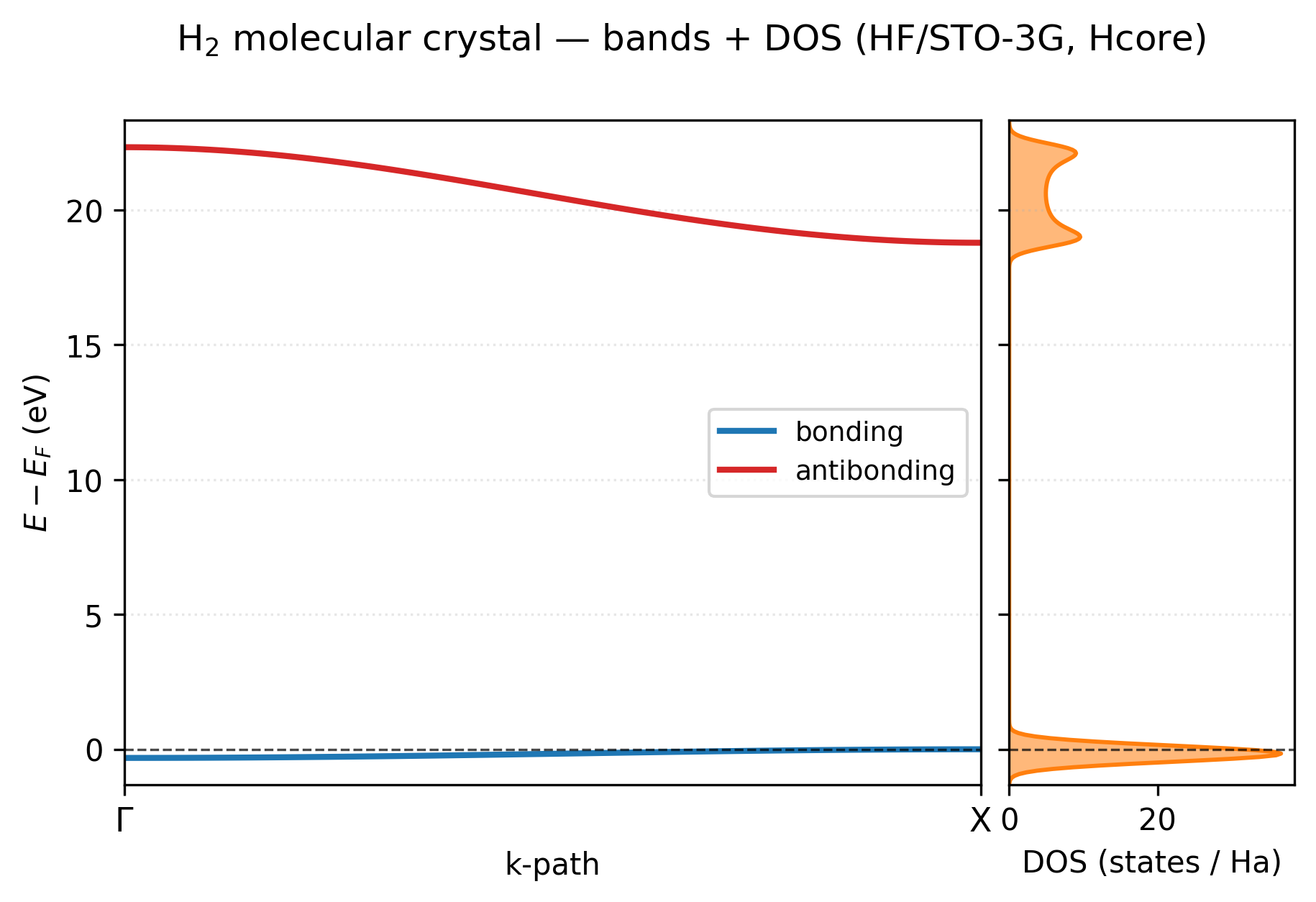
The two Hcore bands are the bonding-like and antibonding-like combinations of the two 1s basis functions. Their width measures how strongly the corresponding Bloch combinations change with k in this model.
Use careful language:
You may say that the Hcore model has two bands and a gap along the sampled path.
You may compare how their dispersion changes when the lattice spacing is varied.
You may not call the plotted separation an RHF or DFT band gap.
You may not infer a global gap solely from one path unless that path includes the relevant extrema.
bands.e_fermi is the highest occupied sampled eigenvalue for this even,
closed-shell electron count. It is a convenient plot reference, not a
finite-temperature chemical potential.
On a dim=1 cell the nuclear attraction in Hcore is a bare lattice sum that
grows logarithmically with the lattice-sum cutoff, so the absolute band
energies, and bands.e_fermi with them, shift rigidly when the cutoff
changes. For this chain the lower band at \(\Gamma\) moves from -2.276 Ha to
-4.004 Ha as cutoff_bohr and nuclear_cutoff_bohr (both passed through
lattice_opts) go from 15 to 200 bohr, while its width along
\(\Gamma\rightarrow X\) settles at 0.0122 Ha and the gap at \(X\) changes by about
3 mHa. Read widths and gaps from this model, not absolute positions. The same
divergence is why a dim=1 cell has no self-consistent route yet: a wire that
needs SCF bands is run as a dim=3 cell with transverse vacuum, as in
Periodic HF.
Theory
Three pieces of machinery sit behind the exercise above: the Bloch eigenvalue problem that produces one set of band energies per \(\mathbf k\), the choice of a path through high-symmetry points along which to display them, and the Gaussian broadening that turns a discrete set of sampled eigenvalues into a density of states. The periodic-HF tutorial derives the first of these in full (Bloch’s theorem); here they are stated in the form the code uses.
The Bloch eigenvalue problem. Bloch’s theorem lets every one-electron state of a crystal be labelled by a band index \(n\) and a crystal momentum \(\mathbf k\) in the first Brillouin zone. Expanding the crystalline orbital in Bloch sums of the atom-centred Gaussians \(\chi_\mu\) of the reference cell gives, at each \(\mathbf k\) separately, a generalised eigenvalue problem of the size of the unit-cell basis,
where \(\mathbf H(\mathbf T)_{\mu\nu} = \langle \chi_\mu(\mathbf r)\,|\,\hat H\,|\,\chi_\nu(\mathbf r - \mathbf T)\rangle\) is the real-space lattice block between the reference cell and the cell translated by \(\mathbf T\), and \(\mathbf S(\mathbf k)\) is the same Fourier sum of the overlap blocks. The eigenvalues \(\varepsilon_n(\mathbf k)\), followed continuously in \(\mathbf k\), are the bands; a band’s dispersion (its width \(W_n\)) measures how strongly the lattice blocks with \(\mathbf T \neq 0\) couple neighbouring cells. In this tutorial \(\hat H\) is the core Hamiltonian, so the blocks are kinetic plus nuclear attraction only; for an HF or KS band the same equation is solved with the converged Fock or Kohn-Sham operator, which is why the route-specific helpers listed above insist on the SCF operator rather than a reconstruction. The Bloch sum of the resulting orbital is the expression shown in the next section.
High-symmetry paths. Bands are functions on a three-dimensional zone,
but they are plotted along one-dimensional paths through points whose
little group (the symmetry operations that leave \(\mathbf k\) fixed up to a
reciprocal-lattice vector) is largest: \(\Gamma\) at the centre, \(X\), \(L\), \(K\)
and the rest on the zone surface, with the standard names and coordinates
tabulated per Bravais lattice by Setyawan and Curtarolo (2010) and Hinuma
and co-workers (Hinuma, Yoyo, Pizzi, Giovanni, et al. (2017). *Band structure diagram paths based on crystallography.* Computational Materials Science, **128**, 140–184. doi:[10.1016/j.commatsci.2016.10.015](https://doi.org/10.1016/j.commatsci.2016.10.015), which KPoints.band_path
follows). Band extrema and degeneracies are forced onto these points by
symmetry, so a path through them shows the features that matter; it does
not sample the zone uniformly, which is why a global gap cannot be read off
one path unless the path contains the relevant extrema, and why the DOS is
computed on a separate uniform mesh.
DOS and broadening. The density of states counts eigenvalues per unit energy per cell, \(D(E) = \sum_n \int_{\mathrm{BZ}} \delta(E - \varepsilon_n(\mathbf k))\,\mathrm d^3k / \Omega_{\mathrm{BZ}}\). On a finite mesh the integral becomes a weighted sum and the delta function must be replaced by a normalised Gaussian of width \(\sigma\),
so that each band state contributes unit area and \(\int D(E)\,\mathrm dE\) equals the number of bands. The broadening is a display parameter, not a physical one: it hides the discreteness of the mesh, and the honest order of operations is to converge the mesh first (the sampled eigenvalue distribution must be stable) and only then choose the smallest \(\sigma\) that gives a smooth curve, as the convergence section below spells out. For metals the same sampled eigenvalues feed the Gilat-Raubenheimer net, which integrates the linearised bands analytically per microcell and needs no \(\sigma\) at all.
See the endpoint orbitals
The accompanying plot evaluates the bonding-like and antibonding-like Hcore crystalline orbitals at \(\Gamma\) and \(X\):
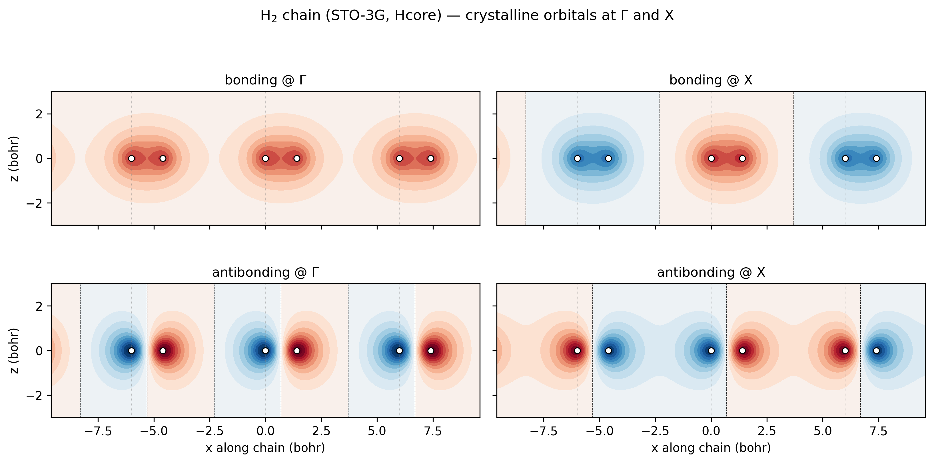
H2-chain Hcore crystalline orbitals at the two path endpoints. Gamma repeats the same phase in every unit cell; X alternates the phase between cells.
The orbital satisfies the Bloch sum
At \(\Gamma\), the phase factor is one. At the 1D zone boundary \(X\), adjacent translations acquire alternating signs. The difference explains why the same local AO combination can have a different energy at the two endpoints.
The maintained generators are:
Converge the mesh before broadening
Repeat the DOS calculation with [40, 1, 1], [80, 1, 1], and
[160, 1, 1]. Compare peak positions and the integrated area. Then hold the
converged mesh fixed and compare sigma=0.005, 0.01, and 0.02 Ha.
The order matters:
Mesh convergence determines whether the sampled eigenvalue distribution is stable.
Broadening determines how that stable distribution is displayed.
Increasing sigma until spikes disappear can conceal an under-sampled mesh.
It does not improve the Brillouin-zone integration.
Change the lattice spacing
Repeat the exercise with x lattice lengths of 5, 6, and 8 bohr while keeping the H-H bond fixed at 1.4 bohr. As neighboring molecules separate, intermolecular coupling weakens and the bands should generally narrow in the Hcore model.
When comparing the three calculations, keep the path resolution, DOS mesh,
basis, and sigma fixed. Record the bandwidth as
This is a controlled illustration of dispersion. It is not a prediction of whether the interacting chain is metallic or insulating.
Add the runner’s QVF diagnostic spectrum
The high-level periodic runner adds total DOS and atom/angular-momentum PDOS to
the default QVF archive. dos_kmesh controls the independent post-SCF mesh:
import vibeqc as vq


def run_bulk_scf_with_dos(system, basis):
    return vq.run_periodic_job(
        system,
        basis,
        method="RKS",
        functional="pbe",
        kpoints=[4, 4, 4],
        dos_kmesh=[12, 12, 12],
        output_qvf=True,
        output="output-bulk-pbe",
    )
Open the resulting QVF in vibe-view to inspect the total and projected DOS, but identify the operator before interpreting it. The current RKS/UKS QVF path reconstructs an operator from the converged density without the exchange-correlation potential. The restricted path also applies full exact exchange. It is therefore a diagnostic spectrum, not the converged Kohn-Sham spectrum, and must not be used for a quantitative DFT band or DOS claim.
For self-consistent bands along a path, use the helper belonging to the SCF
route, such as band_path_eigenvalues for GPW/GAPW,
aiccm2026dev_b_band_structure for AICCM2026DEV-B, or
vibeqc.periodic.ccm.ccm_band_structure for the CCM A stream. The generic
band_structure function is the advanced entry point when your workflow owns
real-space Fock and overlap lattice blocks.
Do not assume a generic SCF result has fock_real or overlap_real
attributes. See the programmatic SCF route table.
CPU time and memory
The Hcore exercise skips SCF and solves one generalized eigenproblem at every sampled k point. Its leading timing trend is
with serial matrix workspace near \(\mathcal{O}(N_\mathrm{bf}^2)\). A self-consistent calculation adds the cost and memory of its SCF route before this spectral post-processing.
Measure CPU time, wall time, and peak RSS together. Record the basis count, path points, SCF mesh, DOS mesh, broadening, threads, host, and version so the comparison can be reproduced.
Next
Projected DOS for Mulliken channel weights and QVF diagnostics.
COOP and COHP for resolving the same states into bonding and antibonding contributions between atom pairs.
k-point sampling for mesh generation and convergence.
Smearing for metals and fractional occupations.
Periodic orbital cubes for a spatial view of selected crystalline orbitals.