Reading a .qvf in the terminal, over SSH

Source commands on this page run from the separate vibe-view checkout. Clone mpei/vibe-view and follow viewer setup. Its .venv, scripts/, and electron/ belong to that repository; vibe-qc does not contain or install the viewer.

You will learn: how to inspect a complete vibe-qc calculation (structure, orbitals, band structure, spectra, convergence, provenance) without a browser, a display server, or copying files back to your laptop.

Why: the machine that produces a .qvf is usually not the machine you are sitting at. vibe-view open needs a browser and an OpenGL context; vibe-view capture needs OpenGL too, and then you still have to move the PNG. Terminal mode needs neither. It is a software rasterizer written in numpy that draws into Unicode braille characters, so it runs on a bare login shell on a compute node.

Prerequisites:

• vibe-view installed on the machine holding the .qvf. The core profile is enough for vibe-view show; install the terminal profile for the interactive vibe-view tui command:

  ./scripts/install.sh --extras tui
  source .venv/bin/activate
  

  If the checkout environment already exists, use ./scripts/update.sh --skip-git --extras tui instead. The distribution is not on PyPI, so a bare pip install 'vibeview[tui]' does not resolve.

• A terminal that speaks 24-bit colour and has a font with braille coverage. Most modern terminals and monospace fonts do; if the glyphs come out as boxes, add --mode half to every command below and the pictures switch to block characters.

Time to complete: about 10 minutes.

Note

Terminal mode and MolTUI solve overlapping problems from opposite ends. MolTUI is a general terminal viewer for the formats the field already uses (.molden, .cube, .xyz, .xsf), so it reads output from any code. Terminal mode reads .qvf and only .qvf, but because a QVF is one self-describing archive it can show you the band structure, the SCF trail, the charges and the citation bundle from the same file – not just the geometry. Use MolTUI when you have loose files from mixed sources; use terminal mode when you have a QVF.

1. Produce a .qvf worth looking at

Any run_job / run_periodic_job call emits one by default. Keep output_qvf=True explicit when the archive is a required deliverable. This water job writes most of the section kinds terminal mode can draw:

# input-water.py
from vibeqc import Atom, Molecule, run_job

mol = Molecule([
    Atom(8, [0.0,  0.00,  0.00]),
    Atom(1, [0.0,  1.43, -0.98]),
    Atom(1, [0.0, -1.43, -0.98]),
])

run_job(
    mol,
    basis="6-31g*",
    method="rks",
    functional="PBE",
    optimize=True,             # trajectory section
    hessian=True,              # vibrations + IR spectrum
    output="water",
    output_qvf=True,           # default, kept explicit here
    write_cube=["density", "homo", "lumo"],  # embeds volumetric grids
    write_molden_file=True,    # embeds wavefunction.gto + the MO blobs
)

<vibe-qc-checkout>/.venv/bin/python input-water.py     # -> water.qvf

Use the vibe-qc interpreter for the calculation even if the active shell is the dedicated viewer environment. The two environments meet at water.qvf.

2. Look at it without leaving the shell

vibe-view show water.qvf

That prints one frame, the structure framed and shaded, then exits. The camera fits the molecule to your terminal’s actual size.

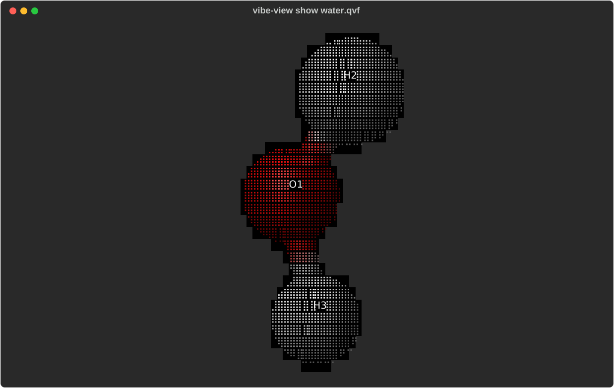
vibe-view show water.qvf --labels. Atoms are drawn as analytically shaded spheres and bonds as split-colour cylinders, packed into Unicode braille cells at two dots across by four down, so an 80x24 terminal is a 160x96 pixel canvas.

Everything about the render is a flag:

vibe-view show water.qvf --representation spacefill
vibe-view show water.qvf --rotate -30,45,0 --labels
vibe-view show water.qvf --size 120x40

Because it exits, it composes like any other command:

vibe-view show water.qvf | less -R        # colour survives the pipe
vibe-view show water.qvf --plain > frame.txt
watch -c -n2 'vibe-view show running.qvf' # crude live monitor

3. Read the metadata before the picture

--info prints provenance, run lifecycle, and the section inventory, which is the fastest way to find out what a calculation actually produced:

vibe-view show water.qvf --info

Archive
path                   water.qvf
qvf version            1
producer               vibe-qc

Provenance
basis                  6-31g*
functional             PBE
method                 rks
scf_converged          True
scf_energy             {'value': -76.38..., 'units': 'Eh'}

Sections
id            kind              status    note
structure     structure         rendered
density       volume.density    rendered
homo          volume.orbital    rendered
lumo          volume.orbital    rendered
wavefunction  wavefunction.gto  rendered
traj0         trajectory        rendered
vib           vibrations        rendered
ir            spectra.ir        rendered
citations     citations         rendered
scf_history   scf_history       rendered

The status column comes straight from vibe-view’s kind registry, so a section the viewer cannot draw still appears, with the honest reason: not yet rendered is a different statement from unsupported.

4. Orbitals and densities

For a precomputed volume.orbital or volume.density, point --section at the stored volume. Signed orbitals get both lobes; the isovalue is yours to choose:

vibe-view show water.qvf --section homo --isovalue 0.05
vibe-view show water.qvf --section homo --isovalue 0.02 --representation licorice

Lowering the isovalue grows the surface. A licorice or wireframe representation keeps the atoms from hiding inside it.

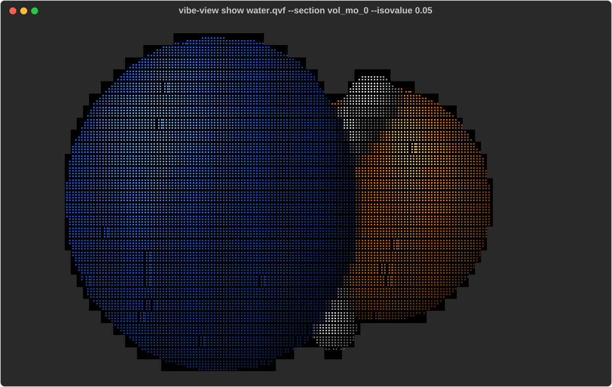
A molecular orbital at isovalue 0.05, licorice representation. Signed fields get both lobes, orange for positive and blue for negative, depth tested against the atoms.

The isosurface itself comes from VTK’s marching-cubes filter, which is pure computation: no render window, no GL context. That is the only place terminal mode touches VTK at all.

The embedded wavefunction.gto section is more powerful: it carries the basis and every MO coefficient row, so the interactive TUI can sample an orbital that was not written as a cube. Start the TUI and move to the desired wavefunction set with Tab:

vibe-view tui water.qvf

The default orbital (the frontier when one is well-defined) appears immediately over the geometry. A surface table opens on the right:

1. Use Up/Down to highlight an orbital.

2. Press Enter to sample and render it. A mouse click on a row does the same thing.

3. Use n/p when you only want to step through orbitals.

4. Use i/I to lower/raise the contour and o to hide/show it.

5. When the archive declares electron-occupation semantics, highlight Total density, or press D, to compute the density. Natural transition orbitals declare transition weights instead, so that row is deliberately absent. An unmarked legacy natural set still renders its individual orbitals but not a guessed density. On an unrestricted wavefunction, highlight Spin density alpha - beta or press S for the signed spin density.

Every archived wavefunction set gets its own table and remembered selection. That includes canonical MOs, alpha/beta unrestricted MOs, natural orbitals, and localized orbitals such as IBO or Boys sets. Localized rows are labelled by their atomic centres instead of a fake energy: a localized orbital is a unitary mixture and is not energy ordered. Natural-orbital rows emphasize occupations. The status line always names the exact rendered row, spin, and isovalue.

On-demand sampling uses a terminal-sized 48 x 48 x 48 grid. The first render of a large basis can take a moment; stepping back to an already sampled row uses the cache. A contour that crosses only one sign legitimately shows one lobe. If no value reaches the chosen isovalue, the geometry stays visible and the status line tells you to lower it with i.

The evaluator covers s, p, d, and f basis shells (l <= 3). It warns in the status line if a selected orbital has significant g-or-higher weight, because that surface is incomplete. Periodic archives expose real Gamma-point fields from central-cell AOs; image-AO tails are not included. The QVF wavefunction contract records the precise limits.

5. Charts

The chart-shaped kinds go through the same command:

vibe-view show water.qvf --section ir            # stick spectrum + envelope
vibe-view show water.qvf --section scf_history   # |ΔE| on a log axis

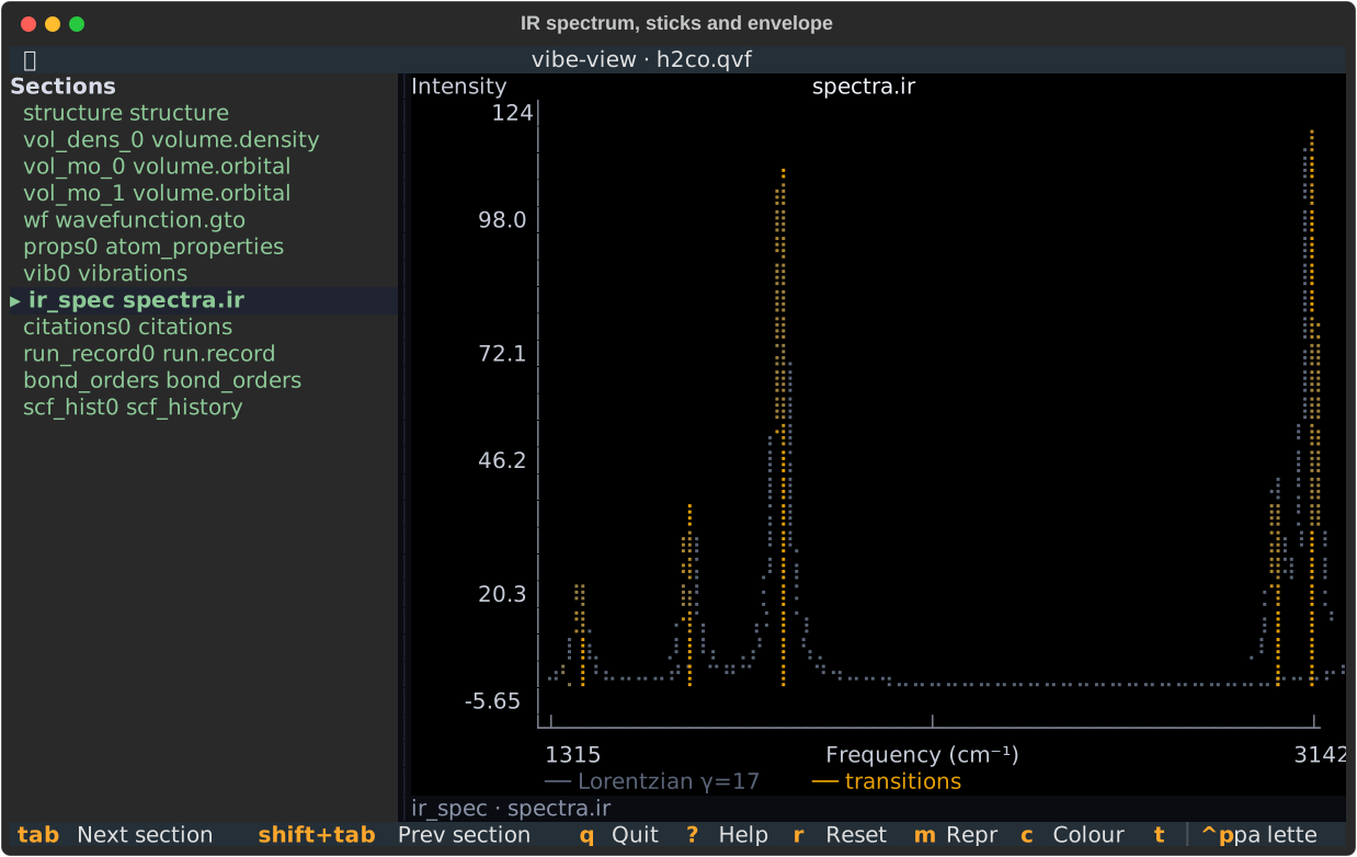
An IR spectrum in the viewport: computed transitions as sticks, with a Lorentzian envelope drawn under them and named in the legend so the convenience is never mistaken for the data.

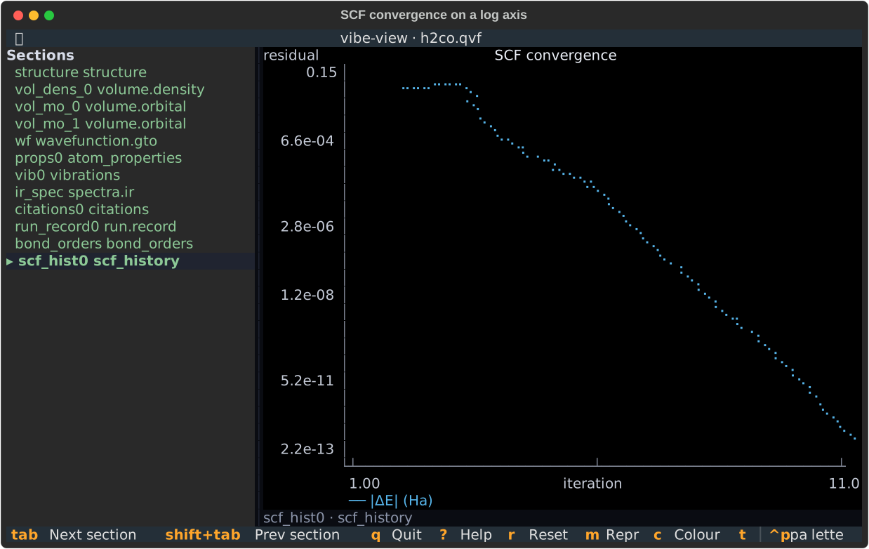
SCF convergence. |dE| on a log axis whose limits are taken after the transform, which is what keeps the converging tail on the plot instead of clipping the very part worth looking at.

Axis conventions follow the interactive Plotly renderers, so a terminal chart and a browser chart tell the same story. In particular, bands and DOS are Fermi-referenced only when E_F falls inside the data window, and are labelled absolute (naming E_F) when it does not.

6. Trajectories and normal modes

Animated kinds take a --frame:

vibe-view show water.qvf --section traj0 --frame 0
vibe-view show water.qvf --section traj0 --frame 8
vibe-view show water.qvf --section traj0 --chart   # the energy profile instead

A trajectory and a reaction path are both geometry and an energy curve; --chart picks the curve.

7. Everything at once

vibe-view show water.qvf --all --plain > report.txt

Renders every graphable section in a reading order, one after another. Useful as a build artefact or attached to a job’s log.

8. The interactive viewer

For browsing rather than checking one thing:

vibe-view tui water.qvf

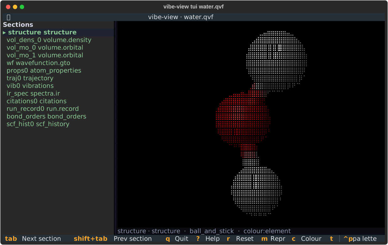
vibe-view tui water.qvf. The section browser lists every section in the archive with its status from the kind registry, so a section the viewer cannot draw still appears with an honest reason rather than being hidden.

Section browser on the left, viewport in the middle, status line naming what you are looking at. Press ? for the full key map; the essentials:

Tab	next section
arrows / h j k l	rotate
+ -	zoom, r to reset
m / c	representation / colour scheme
i I	isovalue down / up
Up Down, then Enter	choose and render a wavefunction surface row
n / p	previous / next orbital while a wavefunction is active
D / S	total density / unrestricted spin density
Space	play an animation
t	data table for the current section
q	quit

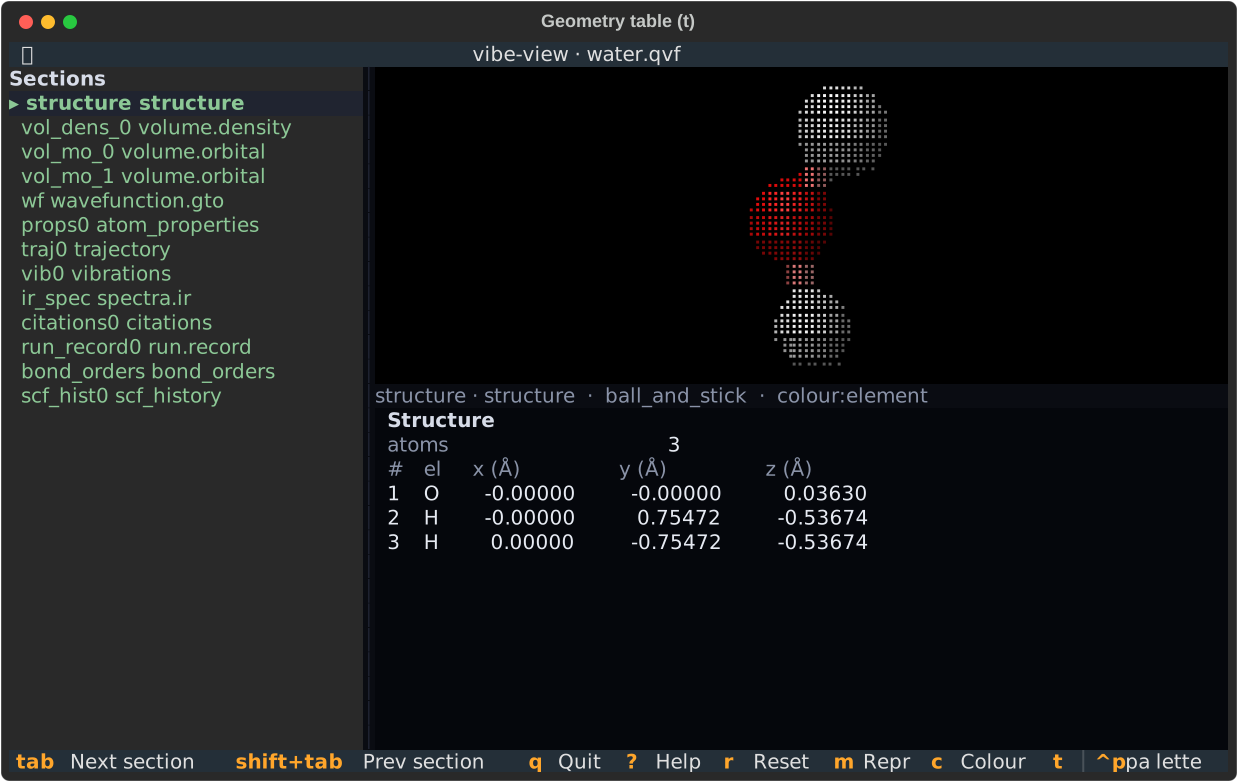
t opens the data table for the current section. On a structure that is the geometry: cell parameters when periodic, Cartesian coordinates, and the bond list with orders and lengths.

9. Periodic systems

Cell edges are drawn only along axes flagged periodic (a 2D slab gets the in-plane parallelogram, never a box around its vacuum), and --replicate respects the same rule:

vibe-view show graphene.qvf --replicate 3,3,1

Bonds crossing a cell face are drawn to the nearest periodic image rather than stretched across the box. This matters more than it sounds: a periodic bond list stores the in-cell index pair, so graphene’s 1.42 Å bonds are listed at separations of 2.84, 3.76 and 5.68 Å. Drawing those endpoints literally produces a hairball; filtering them by length deletes real bonds.

10. From Python

The same renderers are on the public SDK, next to the PNG capture functions:

from vibeview import render_terminal

print(render_terminal("water.qvf", size=(100, 30)))
print(render_terminal("water.qvf", "homo", isovalue=0.03))

# plain=True drops the ANSI colour, for a log file
open("frame.txt", "w").write(render_terminal("water.qvf", plain=True))

A worked script covering the whole surface (representations, orbitals, supercells, charts, text panes, animation) ships at examples/terminal_mode.py:

python examples/terminal_mode.py water.qvf

When terminal mode isn’t enough

It is a reading tool: fast, low-resolution, no setup, works over SSH. For publication figures use vibe-view capture (PNG), the POV-Ray and Blender exporters, or the interactive viewer’s own export. For detailed orbital analysis such as NBO decompositions or ELF/NCI maps, vibe-qc writes .cube and .molden that Multiwfn and VMD read.

Two limits worth knowing before you are surprised by them: a braille cell carries one colour, so two differently coloured atoms sharing a cell blend (zoom in, or use --mode half); and there is no mouse rotation, because terminals report clicks rather than smooth drags.

See also

• vibe-view terminal mode reference: the full option and key reference, including what every section kind shows.

• vibe-view user guide: the interactive browser viewer.

• vibe-view walkthrough: the same archive in the browser, panel by panel.

• MolTUI terminal viewer: the format-agnostic terminal viewer, for loose .molden / .cube / .xyz files.

• QVF file format: what is actually inside the archive being rendered.