Vibrational frequencies¶

The vibrational analysis user guide is the reference for this page: options, output, thermochemistry and every gate. One distinction to have in mind throughout: run_job(hessian=True) builds the Hessian by finite differences of the analytic gradient, and that is the route behind the frequency block of an ordinary job, while the analytic coupled-perturbed Hessians used in the first example below are library functions (vibeqc.compute_hessian_{rhf,uhf,rks,uks}_analytic), not something run_job calls. Both are production routes on the mean-field references (label vocabulary in Methods: theory and status).

vibe-qc has two paths to a Hessian, both wired through the VibeQC ASE calculator:

Analytic CPHF Hessian, the production path. Full coverage for closed- and open-shell HF and DFT (Phase 17a-e):
- vibeqc.compute_hessian_rhf_analytic, closed-shell HF
- vibeqc.compute_hessian_uhf_analytic, open-shell HF
- vibeqc.compute_hessian_rks_analytic, closed-shell DFT
- vibeqc.compute_hessian_uks_analytic, open-shell DFT (LDA, pure-GGA, and hybrid-GGA, e.g. B3LYP, PBE0, all analytic since v0.5.1, which shipped the polarized-GGA fxc kernel completion)
Through the ASE calculator: atoms.calc.get_property("hessian", atoms) dispatches to the right kernel based on the chosen method.
Finite-difference Hessian for any method that produces forces. ASE’s (Larsen, Ask Hjorth, Mortensen, Jens Jørgen, et al. (2017). *The atomic simulation environment - a Python library for working with atoms.* Journal of Physics: Condensed Matter, **29**(27), 273002. doi:[10.1088/1361-648X/aa680e](https://doi.org/10.1088/1361-648X/aa680e)) ase.vibrations.Vibrations displaces each atom in each Cartesian direction (~6N analytic-gradient calls) and builds the numerical Hessian. Slower than the analytic kernel but always available, useful as a sanity check, for methods we don’t have analytic 2nd derivatives for yet, or for tightly integrating with other ASE workflows (NEB, basin-hopping, …).

Both paths give the same products:

normal-mode frequencies (in cm⁻¹)
zero-point vibrational energy
IR intensities (analytic path: Wilson-Decius-Cross, Wilson, E. Bright, Decius, J. C., and Cross, Paul C. (1955). *Molecular Vibrations: The Theory of Infrared and Raman Vibrational Spectra.* McGraw-Hill., from the dipole-derivative tensor; FD path: from finite-difference dipole derivatives)
per-mode atomic-displacement vectors (for animation / vibrational spectroscopy / thermochemistry)

The example below uses the analytic path, that’s the right default for production. A second example at the end of the page shows the FD fallback for reference and for cases where you want the numerical version.

Workflow¶

Three steps:

Optimize the geometry. Hessian at a non-stationary point is meaningless, you’ll get imaginary translations / rotations mixed into the normal modes. Tighten fmax further than for an energy-only optimization (1e-3 eV/Å is a good target) so the gradient is at machine zero before differentiating it again.
Run the analytic CPHF Hessian. One linear-response solve (CPHF for HF, CPKS for DFT) replaces the 6N force calls of the FD path. Cost is dominated by the per-mode SCF response, not by how many atoms there are.
Diagonalize the mass-weighted Hessian to get frequencies and normal modes.

Example: water (analytic CPHF Hessian, RHF / 6-31G*)¶

The script below optimizes water to a stationary point, then calls compute_hessian_rhf_analytic for the frequencies and the zero-point energy, and a finite-difference Hessian with dipole derivatives for the IR intensities (the analytic Hessian result does not carry dipole derivatives):

import numpy as np
import vibeqc as vq

ANG = 1.8897259886                       # Å to bohr

# 1. Build the molecule
mol = vq.Molecule([
    vq.Atom(8, [0.0,  0.0,           0.0]),
    vq.Atom(1, [0.0,  0.7552 * ANG,  0.5863 * ANG]),
    vq.Atom(1, [0.0, -0.7552 * ANG,  0.5863 * ANG]),
])

# 2. Tight SCF + tight optimization first: second derivatives
#    only make sense at a stationary point.
opts = vq.RHFOptions()
opts.conv_tol_grad = 1e-9
mol_eq = vq.optimize_molecule(
    mol, "6-31g*", method="rhf", rhf_options=opts, conv_tol_grad=1e-5,
).system

# 3. Analytic CPHF Hessian, frequencies, zero-point energy
basis = vq.BasisSet(mol_eq, "6-31g*")
result = vq.run_rhf(mol_eq, basis, opts)
hess = vq.compute_hessian_rhf_analytic(
    mol_eq, basis, result, basis_name="6-31g*",
)
freqs = np.real(np.asarray(hess.frequencies_cm1))
zpe_kcal = 0.5 * freqs[freqs > 50].sum() / 219474.6313632 * 627.5095

# 4. IR intensities need dipole derivatives: a finite-difference Hessian
#    (18 displaced gradients for water) with the flag switched on.
fd = vq.compute_hessian_fd(
    mol_eq, "6-31g*", "RHF",
    hessian_options=vq.HessianFDOptions(include_dipole_derivatives=True),
)
ir = vq.ir_intensities(fd)

print(f"Frequencies (cm⁻¹):  {np.round(freqs, 1)}")
print(f"IR intensities (km/mol):  {np.round(ir, 2)}")
print(f"Zero-point energy:    {zpe_kcal:.3f} kcal/mol")

Output on a vibe-qc 0.17.10 development build (HF/6-31G*, optimized to a gradient tolerance of 1e-5 Ha/bohr; the whole script takes about ten seconds on an idle machine):

Frequencies (cm⁻¹):  [   0.     0.     0.     0.     0.     0.  1826.3 4056.  4174.1]
IR intensities (km/mol):  [  0.     0.     0.     0.     0.     0.   110.07  18.29  59.73]
Zero-point energy:    14.377 kcal/mol

The six zeros are translations + rotations (analytic Hessians project them out cleanly, no numerical noise floor). The three real modes are the bend (~1826 cm⁻¹), symmetric stretch (~4056 cm⁻¹), and antisymmetric stretch (~4174 cm⁻¹). The frequencies were cross-validated against ORCA at the same level of theory to 0.5 cm⁻¹ in an earlier release, see Cross-validating against ORCA, Psi4, and PySCF.

Tip

For a vibe-qc-native end-to-end script that writes .molden + ORCA-compatible .hess files and prints the frequency table, see examples/molecular/input-h2o-vibrations.py. The .hess file feeds directly into MolTUI, ChemCraft, Avogadro, and VMD-NMWiz for normal-mode visualization (Viewing geometries, orbitals, and vibrations with MolTUI).

Open-shell DFT (Phase 17e)¶

For open-shell DFT systems (e.g. radicals like OH•), use the UKS analytic Hessian:

result = vq.run_uks(mol, basis, vq.UKSOptions(functional="PBE"))
hess = vq.compute_hessian_uks_analytic(
    mol, basis, result, basis_name="def2-tzvp",
)

Coverage as of v0.5.1 (all paths now shipped):

Method	Closed-shell	Open-shell
HF (RHF / UHF)	✅ analytic (17b-3)	✅ analytic (17c)
LDA / SVWN	✅ analytic (17d)	✅ analytic (17e)
Pure GGA (PBE / BLYP)	✅ analytic (17d)	✅ analytic (17e)
Hybrid GGA (B3LYP / PBE0)	✅ analytic (17d)	✅ analytic (17e-2)

Every closed- and open-shell HF / DFT analytic Hessian path shipped: 17b-3 (RHF), 17c (UHF), 17d (RKS), 17e (UKS LDA + pure GGA), 17e-2 (UKS hybrid GGA, shipped in v0.5.1).

Falling back to finite differences¶

The FD path is still useful as a sanity check on the analytic result, for methods we haven’t implemented analytic 2nd derivatives for yet (e.g. MP2 second derivatives), or for tightly integrating with other ASE workflows. ASE’s Vibrations is the standard tool:

from ase import Atoms
from ase.optimize import BFGSLineSearch
from ase.vibrations import Vibrations
from vibeqc.ase import VibeQC

atoms = Atoms(
    symbols=["O", "H", "H"],
    positions=[
        [ 0.0,  0.00,  0.00],
        [ 0.0,  0.76,  0.59],
        [ 0.0, -0.76,  0.59],
    ],
)
atoms.calc = VibeQC(basis="sto-3g")
BFGSLineSearch(atoms, logfile=None).run(fmax=0.01)

vib = Vibrations(atoms, name="water_vib")  # name= caches per-step force calls
vib.run()
vib.summary()

Typical output (HF/STO-3G, after BFGS to fmax = 0.01 eV/Å):

---------------------
  #    meV     cm^-1
---------------------
  0    0.0      0.0      <- translation
  1    0.0      0.2      <- translation
  2    4.3     34.3      <- rotation
  3    4.6     37.4      <- rotation
  4    0.1i     0.8i     <- near-zero modes (numerical noise)
  5    6.0i    48.8i
  6  268.9  2169.2       HOH bend
  7  513.2  4139.6       symmetric O-H stretch
  8  544.4  4390.6       antisymmetric O-H stretch
---------------------
Zero-point energy: 0.668 eV

The three real internal modes match the chemistry: a bend near 2000 cm⁻¹ and two stretches near 4000 cm⁻¹. HF/STO-3G over-estimates by 15-35%, the usual scaling factor for this level of theory is ~0.89. Multiplying the printed frequencies by 0.89 gives 1930, 3684, 3907 cm⁻¹: the two stretches land within 1 to 4 % of the experimental water frequencies (3657, 3756 cm⁻¹), while the bend stays 21 % above its 1595 cm⁻¹. Bigger basis + DFT gets you closer without the scaling factor.

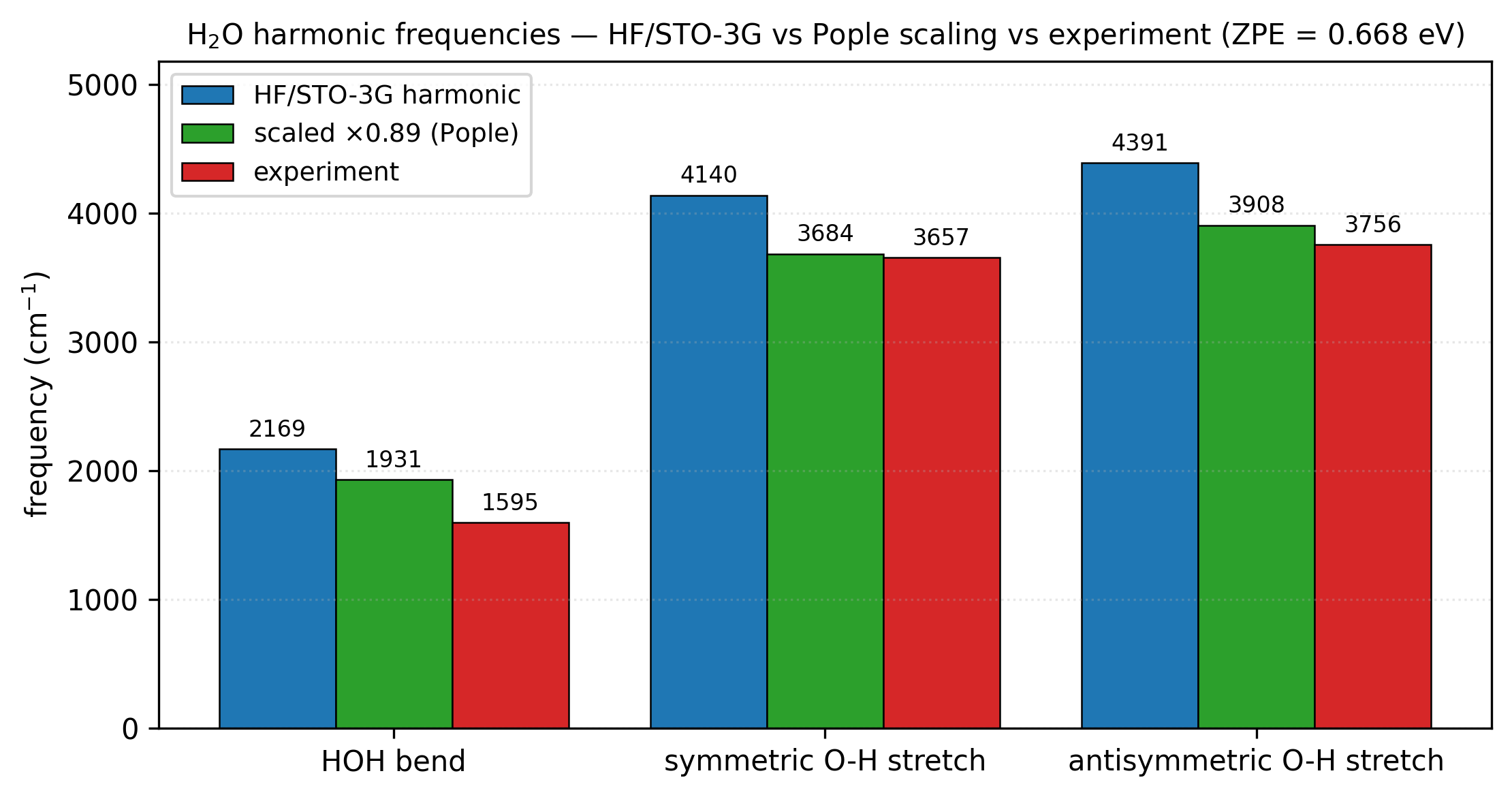
Bar chart of HF/STO-3G harmonic frequencies, scaled (×0.89), and experimental fundamentals for HOH bend and the two O-H stretches. — H₂O harmonic frequencies. **Blue:** raw HF/STO-3G harmonics. **Green:** the same numbers multiplied by the Pople 0.89 scaling factor, which absorbs both the HF over-estimation and the typical anharmonic softening. **Red:** gas-phase experimental fundamentals (NIST WebBook). The two O-H stretches scale to within ~3% of experiment. The bend remains 20% high, since STO-3G is too small a basis to capture the bend angular dependence; cc-pVDZ closes most of the gap, B3LYP/6-31G** (with scaling factor 0.96) closes essentially all of it. Regenerated by `[`examples/plots/water-vibrational-frequencies.py`](https://github.com/vibe-qc/vibe-qc/blob/main/examples/plots/water-vibrational-frequencies.py)`.¶

Pulling the numpy arrays¶

vib.get_frequencies() returns complex frequencies in cm⁻¹ (imaginary ones signal saddle points or numerical noise below the threshold). vib.get_energies() gives meV.

import numpy as np

freqs = vib.get_frequencies()            # complex-valued ndarray
zpe = vib.get_zero_point_energy()        # eV

print("Real frequencies (cm^-1):",
      np.real(freqs[np.abs(np.imag(freqs)) < 1e-6]))
print(f"ZPE = {zpe * 96.485:.3f} kJ/mol")

Animating a mode¶

The three real vibrational modes of H₂O, bend, antisymmetric stretch, symmetric stretch, animated side-by-side, each oscillating along its eigenvector at the analytic-CPHF Hessian frequencies (HF/STO-3G overshoots experiment by ~15-35 %, the expected basis-set + method effect):

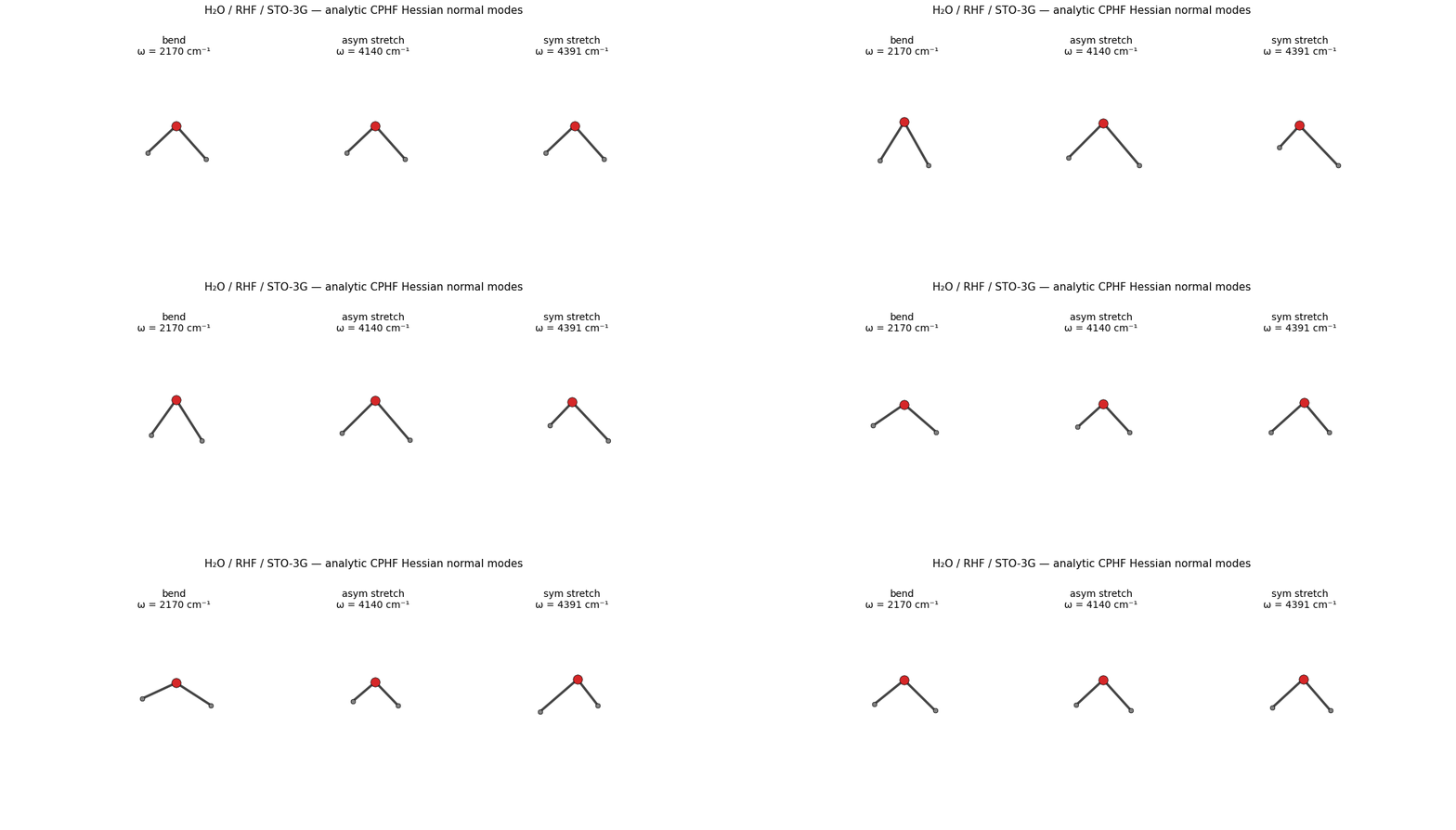
H₂O / RHF / STO-3G, three normal modes oscillating side-by-side: a bend at ~2170 cm⁻¹, symmetric stretch at ~4140 cm⁻¹, antisymmetric stretch at ~4390 cm⁻¹.

The GIF is regenerated by examples/plots/water-normal-mode-animation.py on every release pass; the recipe is straightforward:

Optimize the geometry tightly (fmax = 1e-3 eV/Å) so translations + rotations are at machine zero.
Run the analytic CPHF Hessian via compute_hessian_rhf_analytic, diagonalizing it yields the eigenvalues (squared frequencies) and eigenvectors (cartesian displacement vectors per atom).
For each real mode (drop the 6 modes with |ω| < 100 cm⁻¹, those are translations / rotations), oscillate the atoms along the eigenvector via positions(t) = positions_eq + A · sin(2πt/T) · eigenvector, render each frame with matplotlib’s 3D scatter + line plotting, stitch into a GIF via matplotlib.animation.PillowWriter.

To write an XYZ-frame animation of one mode at a time, ASE’s built-in helper does the same job in two lines:

vib.write_mode(n=8, kT=None, nimages=30)
# -> water_vib.8.traj, open with `ase gui water_vib.8.traj`

You can also render each displaced geometry to XYZ and feed it into your favourite orbital viewer (Jmol, Avogadro, VMD, MolTUI) for publication-quality output. See Viewing geometries, orbitals, and vibrations with MolTUI for the MolTUI workflow that displays vibrations inline in the terminal.

Which surface the frequencies describe¶

run_job(hessian=True) builds the Hessian by finite-differencing an analytic mean-field gradient, and it accepts only RHF, UHF, ROHF, RKS and UKS. A correlated request does not change that. run_job resolves method="mp2" down to the RHF reference its SCF actually runs, then differentiates RHF, so the frequencies, the normal modes and the RRHO thermochemistry all describe the RHF surface even though the job’s reported energy is MP2. The same holds for ccsd, ccsd(t), the DLPNO routes, the coupled-pair and QCI variants, and ovgf.

That is a legitimate and common workflow (a correlated single point with mean-field frequencies), so vibe-qc computes it rather than refusing. It names it, in three places:

the .out frequency block opens with a Surface: line, and when the surface is not the requested method’s it says so outright:

  ## Vibrational Frequencies
  --------------------------
  Surface: RHF/sto-3g  (NOT MP2)
  This job's energy is MP2, but the Hessian finite-differences
  the analytic RHF gradient. The frequencies, normal modes and
  thermochemistry below describe the RHF reference surface;
  no MP2 second derivatives were computed.

the thermochemistry rows name the electronic energy they add the thermal corrections to, E(RHF) + ZPE rather than a bare E(elec) + ZPE. In an MP2 job that number is the RHF energy, not the MP2 total, so if you want the correlated enthalpy you add the printed thermal correction to E(MP2 total) yourself;
the .system manifest gains a [hessian] section and the .qvf archive’s vibrations/metadata.json gains a surface key, both carrying surface_is_requested_method so a consumer can gate on it without reading prose.

A method that resolves to no mean-field reference at all (CASSCF, CISD, CASPT2, NEVPT2, FCI, selected CI, DMRG) has no finite-difference Hessian through run_job. Those jobs report their energy and then say the frequency block was skipped, naming the surface. For CASSCF there is a Python-API route, vibeqc.hessian_casscf.compute_hessian_casscf(mol, basis, active_space), which finite-differences the analytic CASSCF gradient. It is not wired into run_job: its result carries unprojected modes (no translation and rotation projection) and no dipole derivatives, so the frequency table, the RRHO thermochemistry and the QVF vibrations section cannot consume it as it stands.

Caveats¶

Tighten the SCF + the optimization before differentiating. For analytic Hessians, conv_tol_grad = 1e-9 and fmax = 1e-4 Ha/bohr is a sane default. Loose tolerances surface as spurious low-frequency modes (~10-100 cm⁻¹) that wouldn’t be there at machine zero.
FD displacement step matters (FD path only). ASE’s default 0.01 Å is usually fine. If a mode looks noisy, reduce it (Vibrations(..., delta=0.005)) and re-run.
Periodic Hessians are not phonons. run_periodic_job(hessian=True) computes the finite-difference Hessian of the isolated unit-cell molecule, not a phonon calculation of the crystal; see the vibrational analysis guide for the periodic and preview Gamma-point GAPW phonon routes.

Theory¶

The sections below cover the harmonic normal-mode analysis behind the frequencies, where the Hessian comes from in practice (analytic CPHF/CPKS versus finite differences), why harmonic frequencies sit above experiment, and how the IR intensities are computed.

Normal-mode analysis in a nutshell¶

At a stationary point of the Born-Oppenheimer potential-energy surface, the nuclei oscillate around equilibrium. In the harmonic approximation, the PES is truncated to second order around the minimum \(\mathbf{R}_0\):

\[ V(\mathbf{R}) \;\approx\; V(\mathbf{R}_0) \;+\; \tfrac{1}{2} \, \Delta\mathbf{R}^T \, \mathbf{H} \, \Delta\mathbf{R}, \]

where \(\mathbf{H}_{AB}^{ij} = \partial^2 V / \partial R_A^i \partial R_B^j\) is the Hessian matrix of second derivatives (Cartesian coordinates, \(A\) / \(B\) atom indices, \(i\) / \(j \in \{x,y,z\}\)). Substituting into Newton’s equation \(M_A \ddot{R}_A^i = -\partial V / \partial R_A^i\) and decoupling via the mass-weighted Hessian

\[ \tilde{\mathbf{H}}_{AB}^{ij} = \mathbf{H}_{AB}^{ij} \, / \, \sqrt{M_A \, M_B} \]

gives a \(3N \times 3N\) eigenvalue problem (Wilson, E. Bright, Decius, J. C., and Cross, Paul C. (1955). *Molecular Vibrations: The Theory of Infrared and Raman Vibrational Spectra.* McGraw-Hill.) whose eigenvalues \(\lambda_k = \omega_k^2\) are the squared normal-mode frequencies and whose eigenvectors are the mode displacements. Out of the \(3N\) modes, 6 (or 5 for linear molecules) have \(\omega = 0\): three translations and three rotations. The remaining \(3N - 6\) are the genuine vibrational modes.

An imaginary frequency (\(\omega^2 < 0\)) indicates a negative Hessian eigenvalue, the PES curves downward in that direction. At a true minimum there are none. At a first-order saddle point (a transition state) there is exactly one.

Where the Hessian comes from in practice¶

Analytic second derivatives require solving a coupled-perturbed equation (CPHF for HF, CPKS for DFT; Pople, J. A., Krishnan, R., et al. (1979). *Derivative studies in Hartree-Fock and Møller-Plesset theories.* International Journal of Quantum Chemistry, **16**(S13), 225–241. doi:[10.1002/qua.560160825](https://doi.org/10.1002/qua.560160825)), effectively one linear- response solve per perturbation, plus the underlying SCF, and vibe-qc ships them for RHF / UHF / RKS / UKS in Phase 17a-e. The CPHF/CPKS equations read

\[ (\boldsymbol{\varepsilon}_a - \boldsymbol{\varepsilon}_i) \, U_{ai}^{(R)} + \sum_{bj} A_{ai,bj} \, U_{bj}^{(R)} \;=\; -B_{ai}^{(R)}, \]

where \(U_{ai}^{(R)}\) is the orbital response to nuclear displacement \(R\), \(A\) is the orbital-Hessian operator (Coulomb + exchange + XC kernel pieces), and \(B^{(R)}\) contains the skeleton 2nd-derivative integrals. vibe-qc solves these iteratively (Pulay DIIS) and assembles the final 2nd-derivative tensor.

For methods without an analytic implementation today (meta-GGA functionals, MP2), or as a sanity check, vibe-qc falls back to numerical differentiation of the analytic gradient:

\[ \frac{\partial^2 V}{\partial R_A^i \partial R_B^j} \;\approx\; \frac{g_B^j(\mathbf{R} + \delta \hat{e}_A^i) - g_B^j(\mathbf{R} - \delta \hat{e}_A^i)}{2\delta} \]

central differences on the gradient, displacement \(\delta \approx 0.01\) Å. Cost: \(6N\) gradient evaluations per molecule on top of the optimization. Noise floor on the low-frequency modes is set by the SCF force accuracy (~50 cm⁻¹ at the default conv_tol_grad = 1e-6).

Harmonic frequencies vs. experiment¶

The harmonic approximation overestimates fundamental transitions (observed IR peaks) for two reasons:

Anharmonicity. Real potentials are softer than the harmonic fit, the well widens as you climb it. Actual transition energies are \(\sim 3\)-\(5\%\) below \(\omega_\text{harmonic}\).
Method error. HF overestimates frequencies by \(\sim 10\)-\(15\%\); GGA-DFT typically overestimates by \(\sim 2\)-\(5\%\).

The community absorbs both into a single empirical scaling factor: multiply every \(\omega\) by a constant (0.89 for HF/6-31G*, 0.96 for B3LYP/6-31G**, …) before comparing to IR band maxima. Tabulated values for many method/basis pairs live in the NIST CCCBDB; Wong’s 1996 paper (Wong, Ming Wah (1996). *Vibrational frequency prediction using density functional theory.* Chemical Physics Letters, **256**(4–5), 391–399. doi:[10.1016/0009-2614(96)00483-6](https://doi.org/10.1016/0009-2614(96)00483-6)) is the standard reference, updated for many functionals by J. P. Merrick, D. Moran and L. Radom, J. Phys. Chem. A 111, 11683 (2007), doi:10.1021/jp073974n.

IR intensities¶

The integrated absorption intensity of mode \(k\) in the harmonic, double-harmonic approximation is

\[ I_k = \frac{N_A \pi}{3 c^2} \, \Bigl| \frac{\mathrm{d} \boldsymbol{\mu}}{\mathrm{d} q_k} \Bigr|^2, \]

where \(q_k\) is the normal-mode coordinate. Computing this needs dipole-moment derivatives, the “double-harmonic” part because we differentiate both the potential (→ \(\omega\)) and the dipole (→ \(I\)). vibe-qc computes dipole derivatives by finite differences alongside the finite-difference Hessian (HessianFDOptions(include_dipole_derivatives=True)); the analytic Hessian result of the example above does not carry them, so the IR intensities come from the finite-difference route:

fd = vq.compute_hessian_fd(
    mol_eq, "6-31g*", "RHF",
    hessian_options=vq.HessianFDOptions(include_dipole_derivatives=True),
)
print(vq.ir_intensities(fd))
# [  0.  0.  0.  0.  0.  0. 110.07  18.29  59.73]

The first six entries are translations + rotations (zero by construction); the remaining \(3N - 6\) are the per-mode IR intensities in km/mol, the unit IR spectroscopists actually use.

Resources¶

Analytic CPHF Hessian (default): ~250 MB peak RAM, ~5 s on one core (Apple M2 baseline) for H₂O / 6-31G*, a linear-response solve for the \(3N_\text{at}\) nuclear perturbations dominated by the orbital-Hessian application. Cost scales as \(\mathcal{O}(N_\text{bf}^4)\) per CPHF iteration and perturbation, ~\(\mathcal{O}(N_\text{bf}^4 N_\text{at})\) overall.

Finite-difference fallback (e.g. meta-GGAs): ~250 MB peak RAM, ~30 s on one core for H₂O / 6-31G*: 6N = 18 displaced SCFs

one analytic-gradient pass per displacement. Cost scales linearly in atom count via the 6N displacements; quartic in basis size per SCF. Roughly 5-10× more wall time than the analytic path on small molecules.

References¶

Normal-mode analysis, canonical reference. E. B. Wilson Jr., J. C. Decius, and P. C. Cross, Molecular Vibrations: The Theory of Infrared and Raman Vibrational Spectra, Dover (1980; reprint of 1955). The textbook, every subsequent implementation starts from its \(\mathbf{GF}\)-matrix formulation (in internal coordinates; the Cartesian/mass-weighted form above is the modern working version).
HF/DFT scaling factors. M. W. Wong, “Vibrational frequency prediction using density functional theory,” Chem. Phys. Lett. 256, 391 (1996).
Updated scaling factors (multiple functionals). J. P. Merrick, D. Moran, and L. Radom, “An evaluation of harmonic vibrational frequency scale factors,” J. Phys. Chem. A 111, 11683 (2007).
ASE Vibrations. A. H. Larsen et al., “The atomic simulation environment, a Python library for working with atoms,” J. Phys. Condens. Matter 29, 273002 (2017). vibe-qc drives ASE’s finite-difference Hessian through its VibeQC calculator.
Textbook. F. Jensen, Introduction to Computational Chemistry, 3rd ed., Wiley (2017). Chapter 4 covers normal-mode analysis at an operational level.

Next¶

Once you have vibrational frequencies, you can compute thermodynamic functions (ZPE, internal energy, entropy, enthalpy, Gibbs free energy at temperature) via ASE’s IdealGasThermo, see thermodynamics.